Abstract
Our purpose was to develop a fully automatic method to deal with the presence of high levels of noise interfering with quantitative analysis of fast, dynamic mercaptoacetyltriglycine renogram images. Methods: A method based on Legendre polynomials to fit and filter time–activity curves was proposed. The method was applied to a renal database that contains Monte Carlo (MC)–simulated studies and real adult patient data. Clinically relevant parameters such as relative function, time to maximum uptake (Tmax), and half-emptying time (T1/2) were obtained with the proposed method, the 1-2-1 filter (F121) method recommended in the 2018 guidelines of the European Association of Nuclear Medicine, and a state-of-the-art commercial software program (Hermes) currently used in routine nuclear medicine. Results: The root mean squared error between reference time–activity curves and the same curves with Poisson noise added was about 2 times lower for the Legendre method than for F121. The left relative function for MC and patient data was statistically equivalent for Hermes, Legendre, and F121 (P < 0.001). For MC studies, the Legendre technique performed better that the Hermes method regarding the known values of Tmax (P < 0.05), and the T1/2 determination was significantly improved (P < 0.05). For patient data, the Legendre and F121 methods were less influenced by noise in the data than the Hermes method, particularly for T1/2. Conclusion: In dynamic nuclear medicine imaging, Legendre polynomials appear to be a promising, fully automatic noise-removal tool that is routinely applicable, accurate, and robust.
The human body is characterized by a wide variety of dynamic processes with a large spectrum of durations. Nuclear medicine allows the imaging of some of these processes (1). Isotopic renography is one of the oldest nuclear medicine examination techniques (2), has been studied often, and is still the subject of new developments (3). By recording a succession of time-limited images, the uptake and washout of a radiotracer by the kidneys can be followed and quantified. Each image represents only a few seconds of acquisition. In combination with the very low levels of injected activity, the result is very noisy images, even in healthy patients. The noise level can be much higher in many pathologic situations in which kidney uptake is reduced. Besides visual interpretation of the images in cine mode, time–activity curves can be built from the images, and some quantitative parameters can be derived from these time–activity curves, which are a useful tool that will likely be increasingly used and required (4–6). The most used parameters are left relative kidney function (LRF), time to maximum uptake (Tmax), and half-emptying time (T1/2). Noisy images lead to noisy time–activity curves, and reduced accuracy and precision in the values of these parameters are observed (7).
The noise in nuclear detection is Poisson noise, and its control has been and is still challenging. Many postacquisition noise reduction techniques have been explored: conventional low-pass filters, Fourier filtering, wavelets, or heuristic approaches (8,9). In the 2018 European Association of Nuclear Medicine guidelines for renal scintigraphy in adults (6), the recommended noise reduction technique is a filter, based mainly on the works of Fleming (10,11), with a 1-2-1 Kernel (F121) and a variable number of passes as a function of the number of counts in the time–activity curve.
In this study, we explored a noise reduction method based on the finite Legendre transform (FLT), which makes use of Legendre polynomials. Legendre polynomials are orthogonal polynomials. They benefit from the interesting mathematic properties of orthogonal polynomials, and their computation can be fast (12). Although orthogonal polynomials have already been used in nuclear medicine (13), our approach uses sparse Legendre polynomials and offers the possibility of automating the process for choosing the degree of polynomials that allows the root signal of the time–activity curve to be represented while eliminating much of the noise. The technique has been tested using simulated and real adult patient data—and the LRF, Tmax, and T1/2 parameters—and was compared with results obtained with F121 or a commercial software program currently used in clinical routine.
MATERIALS AND METHODS
Ethical Institutional Review Board approval was obtained, and the requirement to obtain informed consent was waived for this study because of its retrospective nature.
The unifying idea of this study was to test and challenge the FLT-based method on a database containing Monte Carlo (MC)–simulated realistic renography images (14) and real adult patient data
The 2018 guideline of the European Association of Nuclear Medicine (6) covers a large number of noise reduction methods for renal scans, of which very few have been implemented in clinical routine; we therefore took the recommended F121 as a baseline for comparison with FLT. We also processed the data using state-of-the-art commercial software. The relative function, Tmax, and T1/2 were obtained with this software; the F121 and FLT techniques were compared, and for the MC data they were also compared with the ground truth.
Legendre Transformation Technique
This work was based on the FLT of generalized functions (15) and relies on the Weierstrass approximation theorem applied in this study to noisy time–activity curves. This theorem states that we can construct a sequence of polynomials On(t) (n = 0,…, ∞) that converge uniformly to any continuous function f(t) on a finite interval  . We may write
 Eq. 1where the An are weighting coefficients. For the Legendre transformation, Equation 1 becomes
 Eq. 2where
  is the Legendre polynomial of order k and the Legendre coefficients L(k) are computed from
 Eq. 3where
  is a normalization factor linked to the Legendre polynomial.
Before the transformation, a rescaling of the f(t) domain [t1, t2] has to be performed on the definition domain of the Legendre polynomial, which is [–1, +1].
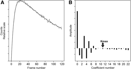
In a preliminary study, a series of pure biexponential curves (Fig. 1A) that mimic, as a first approximation, normal and abnormal kidney time–activity curves was generated. Poisson noise was added to these curves to test the effect of the FLT. A perfect recovery of the original biexponential was achieved when using only a few Legendre coefficients in Equation 2. In the case of noisy biexponentials, the signal and the noise appeared to be mapped to 2 separate spaces (Fig. 1B), and the highest coefficient number (kmax) to use in the limited Legendre transform could be automatically determined by a threshold function based on a ratio of noise to signal. The kmax (also sometimes called cutoff) was applied to the set of Legendre coefficients of the curve, and the inverse Legendre transform was calculated to obtain  :
: Eq. 4which is f with considerable noise removal (Fig. 1A).
(A) Noisy simulated curve (solid) and associated Legendre transform (dashed). (B) Values of 23 first Legendre coefficients obtained using Equation 3 and corresponding kmax.
Applied to real renogram analysis, Equation 4 was the time–activity curve with marked noise removal developed as a sequence of limited Legendre polynomials of degree kmax, with no assumption as to the kind of noise present in the data.
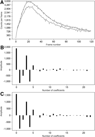
This approach has been tested on MC and patient datasets from the renogram database used further in this study. We found that the Legendre coefficient spectrum always had the same behavior for the type of raw time–activity curve encountered in mercaptoacetyltriglycine studies (Figs. 2 and 3). Starting from the left part of Figures 2B, 2C, 3B, and 3C, it can be seen that the Legendre coefficients decayed to a certain k. This k defined the kmax for the truncated Legendre series expansion of the denoised time–activity curve. The points beyond this kmax were considered to be related to the noise in the raw data.
(A) Raw MC data curves (solid) with corresponding denoised signal by FLT (dashed and dotted). Top curve is left kidney; bottom curve is right kidney. (B) Spectrum of first Legendre coefficients for left kidney in A. (C) Spectrum of first Legendre coefficients for right kidney in A. B and C have same kmax (coefficient number, 16).
(A) Raw patient data curves (solid) with corresponding denoised signal by FLT (dashed and dotted). Top curve is left kidney; bottom curve is right kidney. (B) Spectrum of first Legendre coefficients for left kidney in A. (C) Spectrum of first Legendre coefficients for right kidney in A. In this case, kmax slightly differed between the 2 kidneys: 11 for left and 12 for right.
The kmax was individually and automatically determined on the Legendre coefficient spectrum. The maximum number n of Legendre polynomials to be used was determined by the Runge formula on polynomial interpolation and was related to the total number of points m in the time–activity curve. It is expressed by the following formula: Eq. 5
Eq. 5
An autocorrelation process was applied to the absolute values of the n coefficients, and each component was divided by the factor (2 × k + 1), where k is the kth Legendre coefficient considered. The minimum of this function gave us the kmax value.
Kidney Database
For the following parts of the study, we used a freely accessible online kidney database (www.dynamicrenalstudy.org) that contains MC-simulated studies (14) and real adult patient data.
This MC database was built using the SIMIND MC simulator, a 3-dimensional digital phantom of a human torso (XCAT), and the 99mTc-mercaptoacetyltriglycine pharmacokinetic properties. The tracer pharmacokinetic profile was modeled using a multicompartment model and the following first-order linear differential equation: Eq. 6where
  is the tracer concentration in compartment i at time t,
  the volume of the ith compartment, and
  the transfer rate constant from compartment j to i. The simulation incorporated heart, liver, bladder, and plasma concentration curves. The renal cortex and the medulla were modeled by delay functions to allow for a realistic time distribution. The MC dataset comprised 6 studies based on the same phantom for a total of 30 simulations. Each study represented a specific split function. Images were available for 2 different levels of simulated injected activity (50 and 100 MBq) and for anterior and posterior views, as well as a reference study (RS) posterior view. RS was a simulation without noise, tissue background, and attenuation, giving the actual time-variant tracer distribution (ground truth). Each study was based on the characteristics of its own RS. In all other simulations, a difference in the kidney-to-skin distance was considered. Each simulated dataset consisted of a dynamic renogram acquisition of 120 frames of 10 s and 128 × 128 pixels. The MC study characteristics are summarized in Table 1.
MC Study Characteristics
In addition to the images available in the database, we created a new set of images to which we added Poisson noise on RS in order to compare FLT with the number of coefficients automatically detected and F121 with several passes ranging from 2 to 8. These numbers of passes were chosen to cover all possible values that could be reached by the formula described for this filter in Fleming’s publications (10,11). The root mean squared error between the RS and the RS with the Poisson noise added was evaluated for the 12 simulations.
The patient database was 99mTc-mercaptoacetyltriglycine studies with posterior and anterior projections recorded in a single acquisition. The studies were a 30-min dynamic acquisition of 180 frames of 10 s in 128 × 128 pixels. After browsing through the database, it appeared that the first 20 patients were representative of the clinical cases and the shape of time–activity curves encountered in the database. Only these 20 nondiuretic patient studies were further considered for this study. A partial summary of the clinical diagnosis is available in Supplemental Table 1 (supplemental materials are available at http://jnm.snmjournals.org). Anterior studies were used to assess if the worsening of the signal-to-noise ratio compared with the posterior views would influence the method. The computation of anterior studies was also done for further consideration of a possible geometric mean approach (11).
Regions of Interest (ROIs) and Background Correction
Whole-kidney ROIs and backgrounds were drawn over the kidney using the Hermes renogram analysis software (version 2.6Q; Hermes). For background regions, we used the automated background generated by the Hermes software (lateral, going from the lower to the upper poles). This background was manually corrected for some patient data after discussion with a physician. Thanks to an extra module kindly provided by Hermes, we were able to export the ROIs in extensible-markup-language format and subsequently import them to our in-house–developed software.
Using the study with the 50/50 ratio of the relative function, the ROIs were drawn on the study for which visualization of both kidneys was optimal. This step was done separately for the posterior and anterior views, whereupon the ROIs were propagated to all posterior or anterior datasets. This procedure was possible because the simulation relied on the same anatomic model with different subregional voxel behavior.
The background correction was implemented in our in-house software as described in Hermes (4,16) to avoid any possible bias due to different methods.
Time–Activity Curve Analysis
With the integral method, relative left renal uptake was determined for the interval from 1 to 2 min after injection (4,6). Two time parameters were generated: Tmax and T1/2. Tmax was determined by the frame where the first maximum count was reached. T1/2 was obtained from the time of the first maximum count to the time when the time–activity curve decreased to half this value. There were no differences between the Hermes software and our subroutines for the determination of LRF, Tmax, or the number of counts in the imported ROIs, before application of any FLT or F121 method to the raw data of the MC RS. A maximum difference of 0.1 min was observed in T1/2 but was not significant (R2 = 0.997 and P < 0.001). An extrapolation method based on the center-of-gravity technique was used to obtain the position of T1/2. Approximation and rounding methods are not described by Hermes in its documentation. To ensure the use of identical time–activity curves in Hermes and in our software, no attenuation or decay corrections were applied.
Software Implementation
Reference measurements for LRF, Tmax, and T1/2 were performed with Hermes renogram analysis software. This software extracted the studied parameters from the raw data. The Hermes manual (p43 of Hermes document CD505.5_P31S3V2.6) stated a possible smoothing of the time–activity curve for display purposes only, which “does not affect results.” In-house software was developed in Python (version 3.6) to apply FLT or F121 on the raw time–activity curve and background data before extracting the kinetic parameters. F121 was implemented both for a fixed number of passes and for a varying number of passes as described by Fleming for posterior acquisitions (10,11), with a minimum of 2 passes.
Statistical Analysis
The data were divided into 3 subsets (RS, noisy MC, real patient data), and 3 parameters were analyzed (LRF, Tmax, and T1/2). The mean, SD, range, and percentile were used to describe the spread of the measurements. Agreements between methods were assessed by the Bland–Altman method (17). The slope, intercept, and coefficient of determination were obtained from linear regression for a pairwise comparison of the outcomes of the 3 processing methods. Statistical F tests and t tests were performed at a 5% level of significance (P < 0.05) using XLStat (version 2019.1.3). In the case of multiple comparisons, the Holm–Bonferroni adjustment was applied.
RESULTS
RS with Poisson Noise Added
The mean and SD of the root mean squared errors for the kidney global ROIs between the RS and the RS with added Poisson noise are presented in Table 2. The RMS error was calculated between the RS with noise added, FLT, and F121 for different numbers of passes and the RS as a reference. The RMS error was systematically much lower for FLT than for F121 and was statistically significantly different (P < 0.0001) whatever the number of passes in F121. Moreover, applying FLT on the RS or on the RS with noise led to an exactly identical RMS error; thus, the FLT on noisy curves always converged, whatever the noise, to the same baseline. The performance of each method is shown in Supplemental Figure 1, where the effect of the different filters on the high and low frequencies present in the noisy signal is visible. By lowering the ratio of the signal-to-noise ratio on the RS with added Poisson noise, we observed an increase in the optimal number of passes for F121, as described by Fleming (10), but with an RMS always 2–3 times lower for FLT.
Results for 12 Simulations of RMS Error Between RS and RS with Poisson Noise Added for Different Processing Methods
Noisy MC Studies
There was excellent agreement (Table 3) for the measurement of LRF (P < 0.001) among all 3 methods. The LRF between Hermes and FLT or F121 never exceeded a difference of 2%. Between FLT and F121, there was no difference for 86.7% of the LRF values, and for the other values the difference never exceeded 1%.
Summary Statistics of Linear Regression on MC Data for LRF
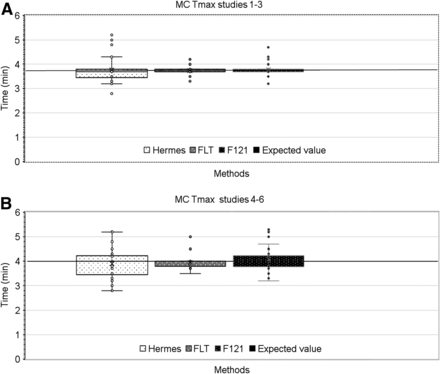
Because simulated Tmax and T1/2 differed after the simulated clearance (Table 1), Tmax and T1/2 results are presented separately for studies 1–3 (clearance, 260 mL/min) and studies 4–6 (clearance, 130 mL/min). Within each group, the mercaptoacetyltriglycine kinetic was the same but the noise level was different. The expected (true) value is indicated in Figure 4. Compared with Hermes outputs, FLT delivered values that were much less dispersed, and the mean value was closest to the expected value. F121 was intermediate between Hermes and FLT.
Box plot of Tmax obtained by 3 methods for left and right kidneys in MC simulations, showing clearance of 260 (A) and 130 (B) mL/min. Horizontal black lines represent expected (true) values given in Table 1.
A statistical analysis was performed on the outputs for Tmax and T1/2 and is presented in Table 4. We used an F test to determine the variance of each pairwise method. The mean and its SD were calculated, and the mean squared deviation from the expected value of the RS was assessed. The ratio of the variance for each pair (F) and its P value were added. Attention must be paid to the fact that T1/2 was computed from the section of the time–activity curve where the signal-to-noise ratio worsens.
Statistical Analysis for MC Data
The analysis of Table 4 showed a mean squared error for Tmax that was systematically at least 2 times lower for FLT than for F121 and reached the level of significance (P < 0.05). For T1/2, mean squared error was also always lower for FLT than for F121, even if the level of significance was not reached for this sample of data. The largest deviations from the expected value (large mean squared error) and SD were observed for Hermes, which computed the parameters from the raw data. A visual example of the discrepancies between the methods for the determination of Tmax and T1/2 is shown in Figure 5.
Fitted time–activity curve obtained with FLT (dashed) or F121 and optimum number of passes (dotted) of raw time–activity curve (solid) and computed kinetic parameters for each method.
Patient Data
For LRF, the data associated with the Bland–Altman plots, reported in Table 5, demonstrated good agreement between F121 and FLT. There were no systematic differences between the values obtained after FLT or F121.
Bias and SD Obtained from Bland–Altman Analysis of Different Parameters for Each Pairwise Method Comparison on Patient Data
For Tmax and T1/2, Bland–Altman plots (FLT vs. F121) are presented in Figure 6 and Supplemental Figure 2, respectively, for both kidneys. The results of the Bland–Altman analysis (bias and SD) are given in Table 5 for the 3 pairwise comparisons. The 2 studies with zero LRF values were excluded from the statistics. The results demonstrate good agreement for Tmax between the FLT and F121 methods in the range of 2–8 min, which is considered the reference range for this parameter (18). The largest differences appeared mainly for abnormal kidneys with a Tmax above 10 min. This observation also holds when comparing FLT and Hermes.
Bland–Altman plot of agreement between Tmax obtained by FLT and F121 for left (A) and right (B) kidneys in patients.
Kidneys with no measurable function have been discarded from the results for T1/2. However, there were also 15 cases with one kidney (and sometimes both) in which T1/2 was never reached during 30 min of examination. These have been visually checked to verify the consistency of the results. For these cases, FLT and F121 resulted in the same output with no T1/2. In contrast, Hermes provided T1/2s ranging from 10 s to a few minutes in about half these cases. For kidneys with normal behavior (T1/2 around or below 5 min) (18), the Bland–Altman plots show fairly good agreement among all 3 methods, as illustrated for F121 and FLT in Supplemental Figure 2. For T1/2s outside the reference range, the differences between the methods were larger.
DISCUSSION
To reduce the impact of Poisson noise on scintigraphy time–activity curves, we proposed a method based on FLT.
FLT can be compared with the Fourier transformation widely used in nuclear medicine and medical imaging. The Fourier transform of the original signal is first computed. Most of the time—for noise filtering, for example—the number of Fourier coefficients is limited to an upper value, the cutoff frequency. Then, an inverse Fourier transformation delivers the final filtered signal. The same global process applies for FLT (kmax can be seen as the cutoff frequency) but with some advantages, such as the low computational cost and the disappearance of side effects, including phase shift in Fourier. In the FLT method, the amplitudes of the components of the Legendre spectrum varied with the noise in the time–activity curve in a different way (Figs. 1–3). Nevertheless, the FLT processing could be fully automated.
The comparison of the noise reduction between RS and RS with added noise was clearly better with FLT, as the RMS error was about 2 times lower than for F121 (Table 2). Furthermore, the expanded view in Supplemental Figure 1 shows that FLT softened the higher and lower frequencies in the signal, whereas F121 kept the lower ones. For RS, the perfect agreement for LRF, Tmax, and T1/2 between Hermes and FLT could be explained by the Weierstrass theorem, which states that any function can be approached by polynomials as closely as desired.
For MC-simulated data, the expected values are known for the 3 parameters (Table 1), thus permitting an evaluation of the correctness and reproducibility of the 3 methods (Hermes, FLT, and F121). The analysis of the results for LRF showed that there were no significant differences among the methods. The statistical analysis showed excellent agreement between FLT and F121. For Tmax, FLT was the method with the lowest SD and mean squared deviation (Table 4). The systematically lowest mean squared error between the expected and measured values and the statistically significant F test confirmed the better performance of the Legendre approach. The comparison with the Hermes system confirmed that working on raw data can lead to large variations in the results. We observed the largest differences from the expected value for T1/2, especially with the Hermes method (Table 4). The direct determination of T1/2 from the raw data resulted in significant fluctuations in the mean square deviation and a large SD, and there were systematically larger differences between Hermes and FLT or F121. It should also be kept in mind that T1/2 relied on the correct determination of Tmax.
For real patient data, the results obtained for LRF shown in Table 5 were comparable for the 3 methods. The close-to-zero bias for all the pairwise comparisons, the upper and lower levels of agreement, and the confidence intervals in Bland–Altman indicate that the FLT method was at least as reliable as the 2 other methods for this parameter. For Tmax, it was observed on the time–activity curve that the presence of noise misled the Hermes algorithm, leading to the same conclusion as for the MC studies: working on raw data induced greater variation in the results. T1/2 was influenced by the correct evaluation of Tmax, and the discrepancies among the different approaches were observed for time–activity curve with a poor signal-to-noise ratio. When a large (in minutes) difference among the methods was recorded, visual assessment systematically confirmed the better performance of FLT and F121 than of Hermes. The statistical analysis (Table 5) showed no evidence in favor of F121 or FLT for Tmax or T1/2 determination in patients. This observation could result from the restricted number of cases in which a large difference between FLT and F121 was observed. It is interesting that these cases systematically concerned values of Tmax or T1/2 outside the normal range.
One advantage of FLT over F121 is that FLT is fully automatic whereas F121 needs to be adapted—for example, if the geometric mean of anterior and posterior images is used. In this case (11), the formula giving the number of passes should be modified by a factor of  . This modification can be seen in Supplemental Figure 3, where we tested FLT for the geometric mean. Moreover, the degree of smoothing with F121 must be increased when considering deconvolution (10), because of the propagation and amplification of noise in this process. The FLT method does not require such adaptation. In our ongoing work on deconvolution-based analysis of renograms, we effectively observed that no modification of FLT was necessary, and the requisite filtering of the curves before and after deconvolution was reduced to a single operation.
There are limitations to this study. First, the MC simulations in the database contained studies for 2 different clearances and with a varying LRF. However, Tmax values were almost identical, and there were only 2 clearly different T1/2 values. Testing FLT for more MC data with an abnormal Tmax or T1/2 would be interesting. Also applying FLT to other databases of patient renograms, and in particular with children’s data, would be a subject of future work in view of a clinical application of the Legendre method. However, such clinical studies were outside the scope of the present initial work. Regarding the case presented in Supplemental Figure 4, FLT filtered not only higher but also lower frequencies, in contrast to F121. However, this finding raised the question of filtering not only statistical noise but also physiologic noise—a possibility that requires a more in-depth investigation.
As a final general remark, we would like to emphasize that the present study does not relate only to renograms, as other types of quantification procedures in nuclear medicine could be concerned.
CONCLUSION
On MC-simulated data, where the true values were known, the Legendre method was definitively superior. The parameter values were the closest to the expected values, and the dispersion was the lowest. For the patient data, the Legendre method and the method recommended by the European Association of Nuclear Medicine were in good agreement, with the exception of the 2 time parameters seen in highly abnormal kidneys. The other advantages of FLT are the fully automated determination of the degree of smoothing and the independence of the method with respect to the type of analysis considered.
DISCLOSURE
No potential conflict of interest relevant to this article was reported.
Footnotes
Published online Jul. 24, 2020.
REFERENCES
- Received for publication March 5, 2020.
- Accepted for publication May 18, 2020.
