


Abstract
Attenuation, scatter, and blurring are 3 major contributors to SPECT image degradation. Image reconstruction without compensation for these degradations results in reduced contrast and reduced quantitative accuracy. In this proof-of-concept study, we present an efficient postprocessing method to compensate for the scatter and blurring effect in SPECT. Methods: A raw image is first reconstructed with attenuation correction only. Then, a 2-dimensional (2D) point spread function (PSF) in the image domain is estimated to model the scatter and blurring. This spatially variant 2D PSF is fitted with an asymmetric gaussian function. The accuracy of the estimated 2D PSF is compared with that estimated from the Monte Carlo simulations and the scatter response functions in the projection domain. A further-blurring-and-deconvolution method is used to restore images with the spatially variant 2D PSF. Results: The method is tested using computer simulations and a phantom experiment. The preliminary results demonstrate an improvement in image quality, with increased image contrast and quantitative accuracy, and the feasibility of this postprocessing method. Conclusion: We present a proof-of-concept study for a postprocessing method to compensate for scatter and blurring. Our results indicate that the method is a promising alternative to the state-of-the-art compensation methods thanks to its easy and fast implementation.
SPECT images are degraded by attenuation, collimator blurring, detector blurring, and photon scatter. Several studies have shown that compensations for these degradations can improve quantitative accuracy and clinical lesion detectability (1–5). The goal of this study was to develop a new method that compensates for scatter and blurring at a clinically acceptable computer time. Currently, the state-of-the-art compensation method is to model the scatter and blurring in the projector–backprojector pair of an iterative reconstruction algorithm (6–20). Also, preprocessing procedures have been investigated to compensate for these physical degradations: compensation for blurring uses the frequency–distance principle (21–24); compensation for scatter uses energy-distribution–based methods (25–27).
In this paper, we propose a postprocessing method to compensate for scatter and collimator-blurring degradation. Instead of doing the compensation before or during the reconstruction, our method corrects for the scatter and blurring effect in the image domain. The method, which can potentially avoid long compensation times for scatter and collimator blurring, was implemented in 3 major steps. First, the raw image was reconstructed using an iterative algorithm with attenuation correction but without scatter and blurring compensation. Second, the reconstructed raw image, which was contaminated by scatter and collimator blurring, was modeled as a blurred version of the original image by a spatially variant kernel. The kernel was what we call a 2-dimensional (2D) point spread function (PSF). This 2D PSF was modeled with an asymmetric gaussian function. We parameterized this gaussian function with some empiric formulas based on the Monte Carlo simulations. Finally, we used an efficient further-blurring-and-deconvolution method to restore the image.
In our previous research, we reported the symmetry properties of the 2D PSF for circularly symmetric objects in a homogeneous medium (28): because the 2D PSF is rotationally symmetric with respect to the rotation center, the 2D PSF with a constant radial distance would thus have the same shape for all angles but be rotated by a certain angle. This assumption has been used in this study. And because of this symmetric property of the 2D PSF, all simulations for 2D PSF estimations were performed on half the x-axis, significantly simplifying the estimations.
MATERIALS AND METHODS
Monte Carlo Simulations and Experimental Phantom
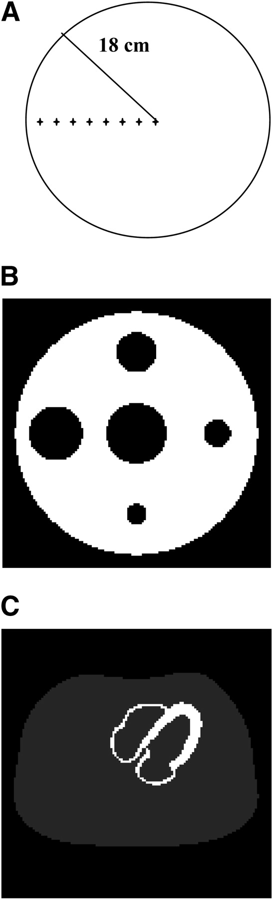
First, to study the variations of the 2D PSF at different point source locations, we simulated 8 line sources at various depths in a uniform water-filled phantom. This cylindric phantom was uniform in the axial direction and had a radius of 18 cm. Figure 1A shows a central slice of the phantom and the point source locations.

Computer simulations. (A) Uniform object used for 2D PSF estimations. Eight point sources with different locations are marked by plus signs. (B) Cold-lesion simulation. This object consists of 5 cylindric cold spots in uniformly attenuating cylinder of uniform activity. (C) Uniform cardiac simulation.
Our scatter compensation method was tested in both computer simulations and a phantom experiment. Two different simulations were performed to validate our postprocessing compensation method in a homogeneous scatter medium. Both objects are centered on the rotation axis of the SPECT camera. For each simulation, the 40 × 40 cm region of the object was digitized onto a 129 × 129 array with a pixel size of 0.31 cm. (An object size of 129 × 129 was chosen to allow placement of the point source in the center of the object.)
The cold-lesion simulation was composed of 5 cylindric cold lesions in a cylindric phantom of uniform activity and attenuation. Figure 1B shows the object and the locations of the cold lesions. The attenuation coefficient for the object was 0.15 cm−1. This simulation was designed to test the accuracy and contrast improvement of our scatter compensation method in the presence of a large source of scattered photons.
The uniform cardiac simulation was a simplified NURBS-based cardiac torso (NCAT) phantom. The attenuator was uniform, with an attenuation coefficient of 0.15 cm−1. The high-activity distribution was confined to the myocardium, as shown in Figure 1C. The intensity ratio of the activity in the myocardium versus background tissues was 5:1.
In all simulations, the Monte Carlo simulation package Simulation System for Emission Tomography (SimSET) (29) was used to generate SPECT data with scatter and collimator-blurring contamination. The SIMSET simulator was chosen because it has reduced variance options with a core module photon history generator. For each simulation, 2 sets of projection data were generated. The first dataset was primary photons representing an ideal data acquisition in which scattered photons are perfectly rejected. The second dataset contained scattered photons only. The detailed simulation parameters are as follows: a 10% energy window around both sides of the primary photon energy peak (140 keV), collimator holes with a thickness of 2 cm and a diameter of 0.14 cm, 300 view angles over the whole 360° scan, and a rotation radius of 20 cm. In each simulation, 1 billion photon histories were generated to yield low-noise projection data.
For the experimental phantom, a flanged Jaszczak hot-rod/cold-sphere phantom was scanned for 1 h using an IRIX SPECT system (Philips). The phantom was filled with water and 799 MBq (21.6 mCi) of 99mTc. Three low-energy high-resolution parallel-hole collimators were used during data acquisition. The rotation radius of the collimators was 24 cm. The data were collected with 180 view angles over a full 360°. The image was reconstructed in a 128 × 128 array with an image pixel size of 0.28 cm.
The Postprocessing Method
Our postprocessing method consists of 3 steps: an iterative algorithm that corrects only for attenuation is used to reconstruct a raw image; a spatially variant 2D PSF is estimated; a further-blurring-and-deconvolution method is developed to restore the image.
Raw Reconstruction.
We start with the SPECT raw projection data. They are contaminated by attenuation and scatter. A reconstructed image, which is here referred to as a raw image, is obtained by implementing an iterative reconstruction algorithm (30–32) that corrects for attenuation only. The imaging geometry can be arbitrary (parallel-beam, fanbeam, cone-beam, and so on). The raw image has been corrected for attenuation but not for scattering and collimator blurring. Our postprocessing method will be applied in the image domain to this raw image.
Collimator Blurring and Scatter Modeling with 2D PSF.
Estimation of the 2D PSF is the essential part of our proposed method. First, we introduce the definition of the 2D PSF. The raw image  is modeled as a blurred version of the original scatter-free and blurring-free image f:
 Eq. 1where the kernel h is what we call a 2D PSF in the image domain and Δ is a small positive number (7 was chosen in this study) representing half the size of the kernel. For each image pixel (i, j), h is a 2D matrix with a size of (2 Δ+ 1) × (2 Δ+ 1). This 2D PSF h is spatially variant, or changes for every image pixel (i, j).
To study the variations of the 2D PSF at different source locations, we model it with a gaussian function: Eq. 2in which the parameter (1 + A) represents the relative amplitude increase because of the scattering (A) and collimator blurring (Eq. 1), (x0, y0) represents the position of the point source, and the parameters FWHMr and FWHMt represent the full width at half maximum (FWHM) of the gaussian function at the radial and tangential directions, respectively. Because the 2D PSF is spatially variant, the parameters A, FWHMr, and FWHMt are the function of the point source location (x0, y0).
This 2D PSF models the scattering and collimator blurring in the 2D image domain instead of in the conventional 1-dimensional projection domain. However, the 2D PSF h can be related to the scatter response functions in the projection domain as follows: Eq. 3where
  represents the scatter response function of a point source located at (x0,y0), and operator FBP represents a filtered backprojection reconstruction with attenuation correction. This approach of obtaining the 2D PSF (referred to as a reconstruction approach), together with the Monte Carlo simulation method, is used to verify our gaussian model of the 2D PSF.
The proposed 2D PSF is also different from the “effective scatter source image” as proposed by Frey and Tsui (12). Both being in the image domain, the effective scatter source image is different for each projection view, and when a projection is applied to this effective image, the estimated scattered projection at this view is obtained; our proposed 2D PSF is a kernel that relates the true image and the raw reconstructed image. Also, we can obtain any projected blurring kernel by performing an attenuated projection operator on the 2D PSF.
Parameterizations of 2D PSF.
In the gaussian model, the parameter A represents the relative magnitude increase caused by scattering. Let fp and fs be the raw reconstructed images from primary and scattered photons, respectively. The value of A can be calculated from the total volume of the image fs with respect to the total volume of the image fp. More details about these 2 images are discussed in Appendix A. We perform the Monte Carlo simulations and the reconstruction approach in Equation 3 to calculate A. The scatter response functions in Equation 3 are estimated using the slab-derived scatter estimation (SDSE) proposed by Frey and Tsui (10). The technique is based on knowledge of the scatter line spread function (SLSF) at different depths inside a slab phantom. The SLSF is fitted with a central gaussian and an exponential as follows: Eq. 4where


In the above expression, D represents the source depth, and s represents the offset from the projected source position at the detector. The scatter response functions are then calculated from the estimated SLSF using a special algorithm, which is discussed in detail in their paper (10).
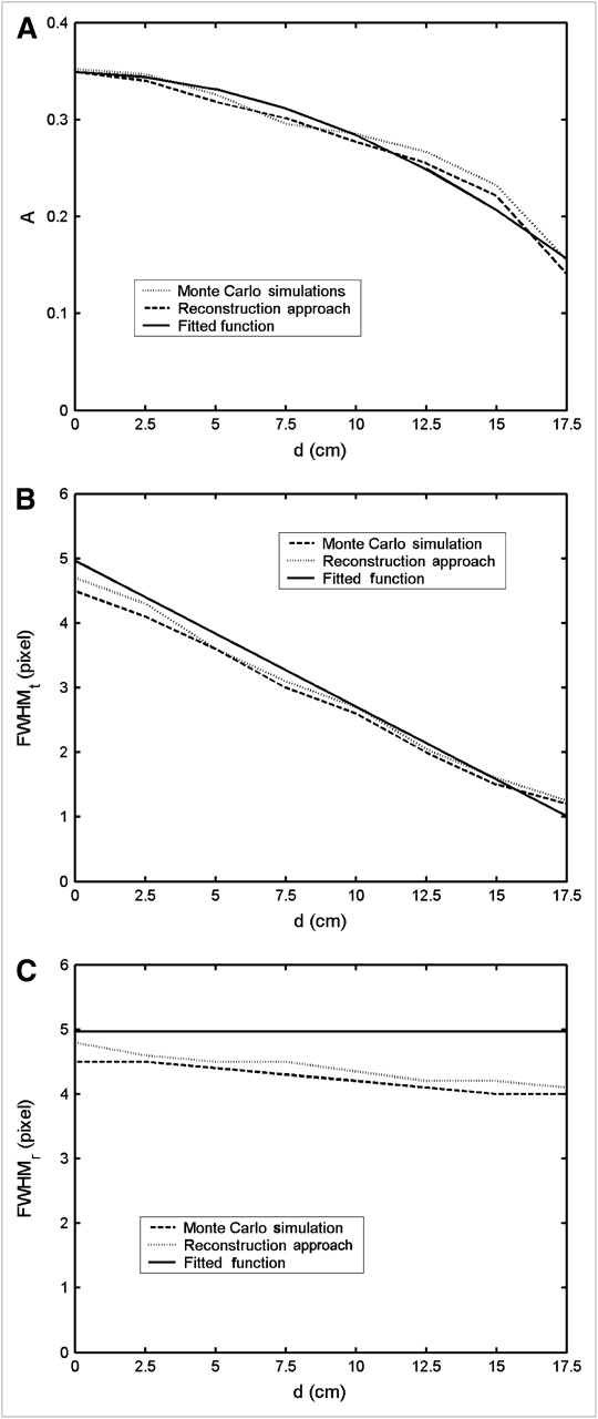
Figure 2A shows the variations in the amplitude A calculated from the Monte Carlo simulations and the reconstruction approach. The decrease in A as the source moves from the center of the object toward the edge can be explained by the fact that the point source close to the center of the object is scattered more than the point source far from the center. We fit A as a function of d, the radial distance from the source to the center of the object, as follows: Eq. 5where A is dimensionless and d is in centimeters. This fitting function of A is plotted in Figure 2A to compare with the results from the Monte Carlo simulations and the reconstruction approach.

Variations of gaussian parameters for 8 point sources as function of radial distance d: relative volume A (A), FWHM in tangential direction of fitted gaussian function (B), and FWHM in radial direction of fitted gaussian function (C).
The FWHM of the gaussian function is determined by the combined effects of collimator blurring and scatter blurring. Because the amplitude of the reconstructed image from the scattered data is small, compared with the reconstructed image from the primary photons (Appendix A), the FWHM of the h depends mainly on the FWHM of the reconstructed image from the primary photons. Therefore, the blurring in the 2D PSF is approximately determined by the collimator blurring. Figure 2B shows a plot of the FWHMt derived from the Monte Carlo simulations and the reconstruction approach. As the source moves from the center of the object toward the edge, the value of FWHMt decreases. In Figure 2C, a plot of FWHMr calculated from these 2 methods is shown. The value of FWHMr barely changes as the source moves from the center toward the edge. Therefore, the FWHMr is modeled as a constant as shown in Equation 7. The constant value in Equation 7 is chosen so that the FWHMr is the same, with FWHMt at the center point (d = 0 cm). The estimation is acceptable considering that the range of values in Figure 2C is within 1 pixel. We then fit the FWHMs of the gaussian function with a distance-dependent model: Eq. 6
Eq. 6 Eq. 7where r is the radius of the collimator hole, l is the thickness of the collimator, μ is the linear attenuation coefficient of the collimator material, D (20 cm) is the distance from the center of rotation to the detector (in cm), and d is the distance from the point source to the center of the object. The comparisons of the fitted FWHMr and FWHMt with the results from the Monte Carlo simulations and reconstruction approach are shown in Figures 2B and 2C, respectively. This model depends only on the point source location and collimator configurations. It is independent of specific objects or patients.
Image Restoration.
Because the 2D PSF is spatially variant, a normal deconvolution algorithm cannot be used. To avoid the long computational time of using iterative restoration algorithms, we developed a further-blurring-and-deconvolution method to restore the image. This method converts the raw image with a spatially variant PSF into a further-blurred image with a spatially invariant PSF and then uses an efficient technique (e.g., a frequency domain filtering) for deblurring.
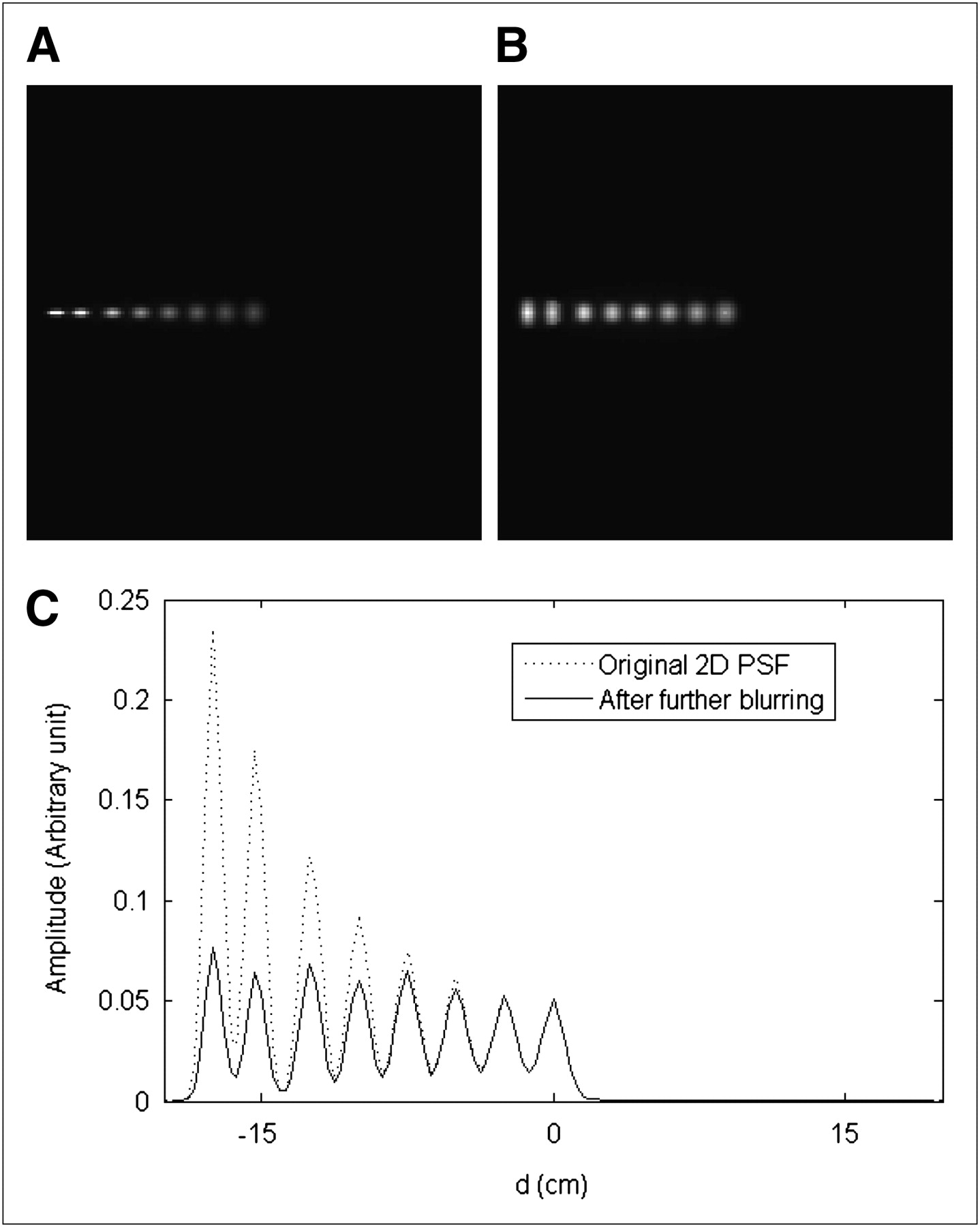
The further blurring is implemented using a rotational convolution. The choice of the rotational convolution is based on the elongated shapes of the 2D PSF along the radial direction and symmetric distributions in the tangential direction, as seen in Figure 3A. Let the raw reconstructed image be  . We rotate the image
  counterclockwise by a small angle θ about the axis of the detector rotation, obtaining
  , and rotate
  clockwise by θ, obtaining
  . If necessary, we rotate the image
  counterclockwise by
  , obtaining
  , and rotate
  clockwise by
  , obtaining
  , and so on. A weighted sum of these rotated images gives a further-blurred image
  :
: Eq. 8where the weighting factors an form a convolution kernel. The sum of an is normalized to 1 to ensure the consistency of the image intensity, and A + 1 is the total volume of the 2D PSF in Equation 2, which is used to normalize the amplitude of the raw image
  with different radial distances d. The weighting factors an, the starting rotation angle θ, and the total number n of sum is currently determined empirically by looking at the further blurred image
  .
.

(A) Spatially variant 2D PSF along radial direction of uniform water filled cylinder; (B) further blurred image using rotational convolution; and (C) profile comparison of 2D PSF before and after rotational convolution.
Now, this further-blurred image  has an approximately spatially invariant PSF and is related to the 2D PSF at the center of the object h0 (Fig. 3B). This approximate method works well for most point sources except for those around the edge of the object. Furthermore, Figure 3C shows the profile comparison in the radial direction of the images before and after this further blurring. This further-blurred image
  can be treated as a spatially invariant blurred image, from which we perform an efficient inverse filtering (e.g., the Wiener filtering) to obtain the restored image f in Equation 1.
Assessment of Restored Image
Sum-squared error (SSE) was used to measure the average discrepancy of the restored image with respect to the original image. It is defined as the averaged sum of the squared pixel difference: Eq. 9where
  and
and  represent the restored value and the true value, respectively, for pixel i, and N is the total number of pixels calculated.
Contrast between activity and background is defined as: Eq. 10where FG represents the average pixel value in the activity distribution and BG represents the average pixel value in the background.
Noise was measured as the SD of pixel counts in the uniform background, normalized by the mean activity of that region.
RESULTS
Verification of 2D PSF Estimations
We compared the 2D PSF for point sources at different locations using the Monte Carlo simulations, reconstruction approach, and our gaussian model. Figure 4A shows profiles along the radial direction of the 2D PSF for 3 different point sources. The radial distances of these 3 points are 0, 7.5, and 15 cm, respectively. Similar comparisons are made in the tangential direction of these 3 points in Figure 4B. The 2D PSF calculated from the Monte Carlo simulations and the reconstruction approach are fit well by the gaussian model, except in the tails. These discrepancies in the tails will be discussed later.
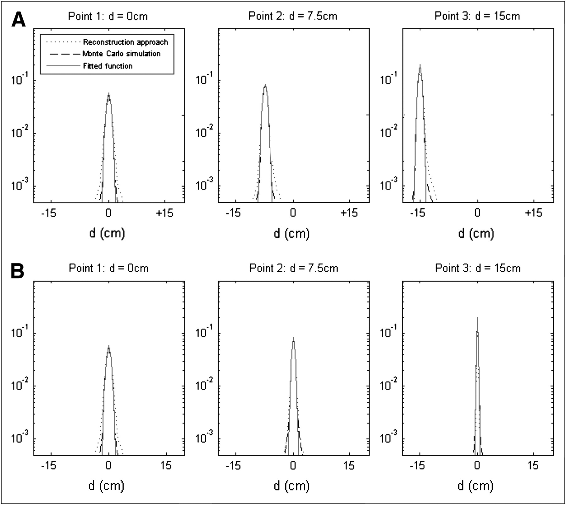
Comparison of 2D PSF calculated from Monte Carlo simulations, reconstruction approach, and fitted gaussian: radial direction (A); tangential direction (B). Profiles are plotted on logarithmic scales.
Computer Simulations
The projection data with scatter and collimator blurring were generated using SIMSET. The maximum-likelihood expectation maximization iterative algorithm was performed for reconstruction with attenuation correction with 30 iterations. The 2D PSF for each simulation was estimated using Equations 5–7. For image restoration, the further-blurred image  was obtained by rotational convolution:
 Eq. 11where
  represents the raw image and
  represents the image rotated by an angle θ. The constant weighting factors were empirically determined according to the shapes of the 2D PSF so that they had a spatially invariant PSF. Wiener filtering was then performed to restore the true image from the further-blurred image
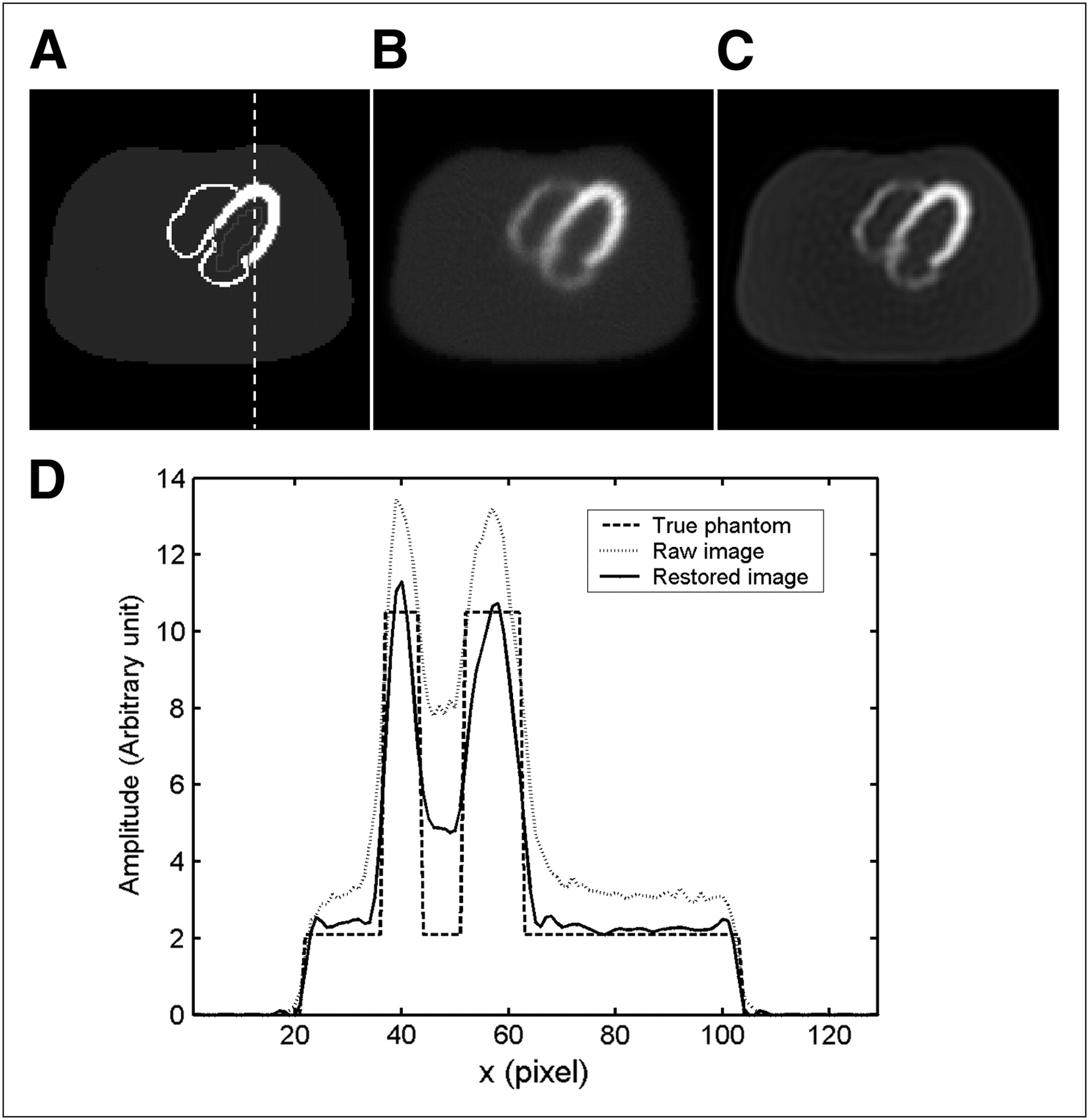
  . For the cold-lesion simulation, Figures 5A–5C show the true image, the raw image reconstructed with attenuation correction only, and the restored image with scatter and collimator blurring compensation using our proposed method. Because of the rotational convolution in which the raw image was rotated to obtain the spatially invariant PSF, the restored image (Fig. 5C) shows some rotational blurring effects. Vertical profiles through the center of the images are plotted in Figure 5D. Similar results for the uniform cardiac simulation are demonstrated in Figure 6.
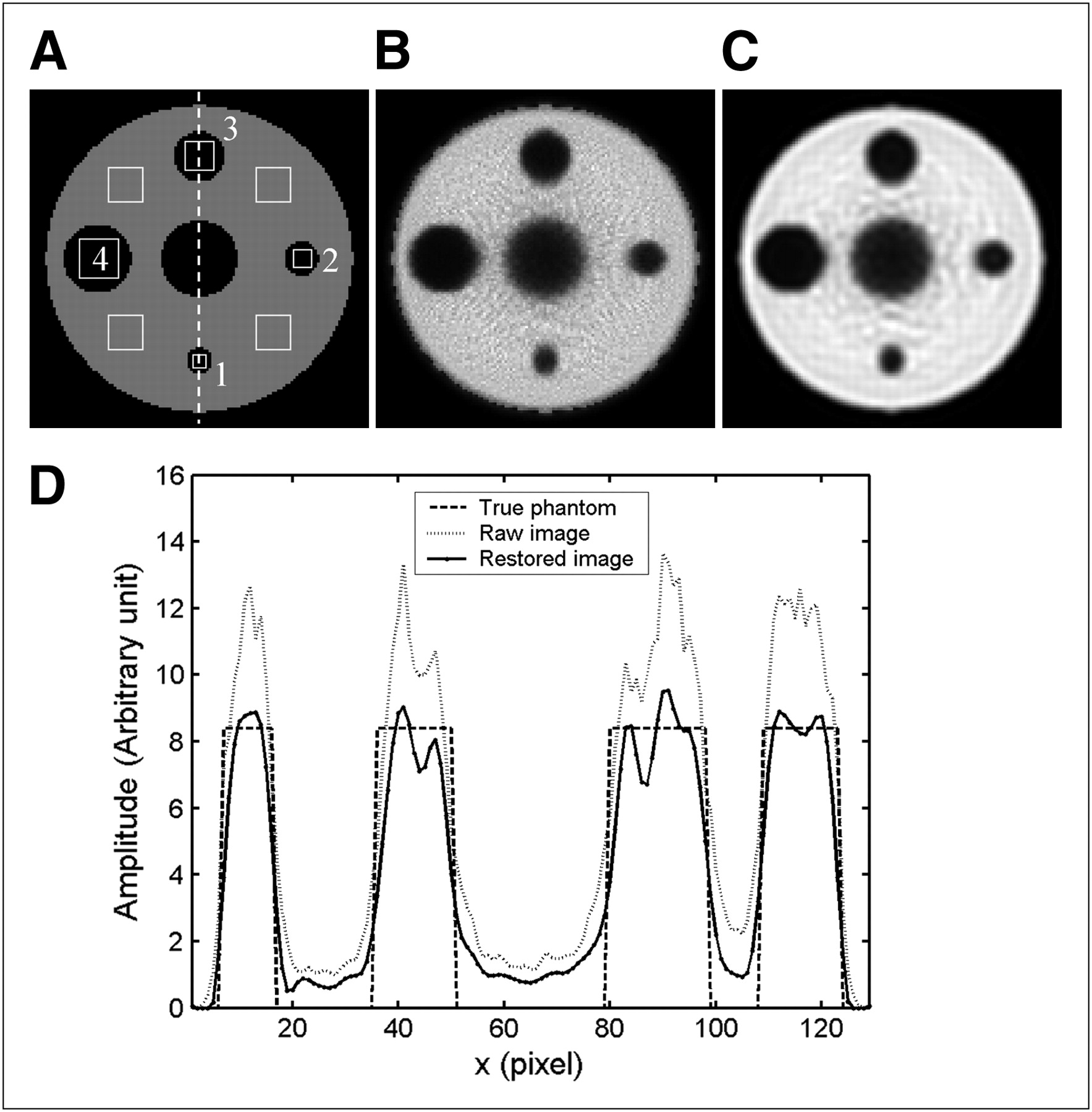
(A) Cold-lesion simulation with locations of region of interest used for contrast analysis, (B) raw reconstructed image with attenuation compensation but without scatter correction, (C) restored image with scatter compensation using our proposed method, and (D) vertical profiles through center of images.

(A) Uniform cardiac simulation with location of region of interest used for contrast analysis, (B) raw reconstructed image with attenuation compensation but without scatter correction, (C) restored image with scatter compensation using our proposed method, and (D) vertical profiles through center of images.
The contrast, SSE, and noise were calculated for all images to illustrate the improvement of quality in the restored image and are demonstrated in Table 1. The regions that were used in the contrast analysis are marked in Figure 6A for the cold-lesion simulation and Figure 7A for the uniform cardiac simulation. After compensation, the quantitative accuracy and contrast were improved. The small increase in the noise level of the cold-lesion simulation may be due to overfiltering in the restoration step.

(A) Jaszczak phantom, (B) raw reconstructed image, and (C) restored image using proposed method.
Comparisons of Image Quality for Computer Simulation Results
Phantom Experiment
The maximum-likelihood expectation maximization iterative algorithm with 50 iterations was used for raw image reconstruction and attenuation correction. Estimation of the 2D PSF was based on the water-filled uniform attenuator and the low-energy high-resolution collimator. For image restoration, the further-blurred image  was obtained by rotational convolution:
 Eq. 12The restored image was obtained after application of Wiener filtering. Figure 7C shows the restored image. The restored image is less noisy than the raw image, as seen by comparing Figure 7C with Figure 7B. This reduced noise may be due to the fact that the Wiener filter is a band-pass filter, and the high frequency noise is suppressed.
DISCUSSION
We have presented a proof-of-concept study of using a postprocessing method to compensate for scatter and collimator blurring in a homogeneous medium. This new method has the potential to reduce computational time, compared with the time required for iterative reconstruction-based methods.
The major challenge of the method is to estimate the 2D PSF in the image domain accurately. We used an asymmetric gaussian function to model the 2D PSF. The total volume 1 + A represents the relative amplitude increase because of scatter and blurring. A is calculated from either the Monte Carlo simulations or the reconstruction approach. The estimated relative total volume is then used in the further-blurring step to adjust the amplitude and obtain the spatially invariant spread function. The width of the gaussian function is largely affected by the collimator blurring. The FWHMs were fitted using a distance-dependent model to calculate the width of the 2D PSF. For image restoration, the width of the 2D PSF at the center of the object is used in the inverse filtering. However, the invariant PSF used in the Wiener filtering was not exactly the same as the 2D PSF h0 at the center of the object: it is narrower in width than that of h0 used in the Wiener filtering. The reason for using this width is to avoid Gibbs ringing artifacts in inverse filtering. Because we are not using the exact width of the estimated 2D PSF, the approximation errors in estimating the 2D PSF do not affect the restored image much. Therefore, our method is robust, and it is not sensitive to the 2D PSF estimation errors. This is the reason why our estimations of the 2D PSF in circularly symmetric objects could tentatively be applied to the uniform cardiac phantom.
Figure 4 showed the comparisons of the 2D PSF calculated using the Monte Carlo simulations, the reconstruction approach, and our gaussian model. The gaussian model does not fit the 2D PSF well in the tails. The discrepancy is small, compared with the amplitude of the 2D PSF, and can be seen only from the logarithmic scale. Also, the gaussian model can be regarded as a fitting for the truncated 2D PSF. A recent study by Beekman's group showed that the truncation of the PSF does not affect the reconstructed image quality much (33). Therefore, the gaussian function is an acceptable fit for the 2D PSF.
For image restoration, a further-blurring-and-deconvolution method is used. The further blurring is implemented using a simple rotational convolution because of the circularly symmetric distribution of the 2D PSF. Although the rotational convolution does affect the spatial resolution, the deconvolution step is there to cancel out the decreased spatial resolution in the first step. Therefore, the method serves the purpose of restoration without undermining the spatial resolution. For a noncircular orbit, rotational convolution may still be used by changing the coefficient an. This noniterative method efficiently restores images with spatially variant PSFs. The advantage of this approach is its fast implementation, compared with conventional iterative algorithms. However, the method is approximate and the rotation angle θ and the weighting factors in Equation 8 are currently determined empirically, raising difficulties for automated implementations. More research needs to be done on this aspect. As the goal of the postprocessing method is to reduce the computational time for the compensation, an efficient restoration method such as this one is desired.
The computational time for this postprocessing compensation method is less than that of the iterative reconstruction-based method. Instead of making a quantitative comparison, which we can do in our further work, we go over the major steps of our postprocessing method and discuss the time consumption. First, the computer time for getting an attenuation-corrected raw image is on the order of seconds for a fast reconstruction (32,34). Then, since we may precalculate the 2D PSF according to our gaussian model and store it in the computer memory, the compensation can be completed within another few seconds for image restoration (i.e., rotational convolution and Wiener filtering). Therefore, the potential of this postprocessing method in reducing computer time is promising for clinical applications.
Our proof-of-concept study is implemented in objects with circular orbits. This simple case gives us an easy approach to estimating the 2D PSF (i.e., the symmetry property mentioned earlier in the paper). This postprocessing method will also apply to objects of complex shape if extra effort is made in estimating the spatially variant 2D PSF. For more realistically noisy data, the methodology of our postprocessing approach will still be valid, expect that we may face more challenges in the image restoration step. Further investigations also include estimating the 2D PSF in an inhomogeneous medium and applying our method to nonuniformly attenuating objects.
CONCLUSION
We have presented a proof-of-concept study for a postprocessing method to compensate for scatter and blurring. Our results indicate that the method is a promising alternative to the state-of-the-art compensation methods thanks to its easy and fast implementation. Further development is encouraged and currently under way.
APPENDIX A
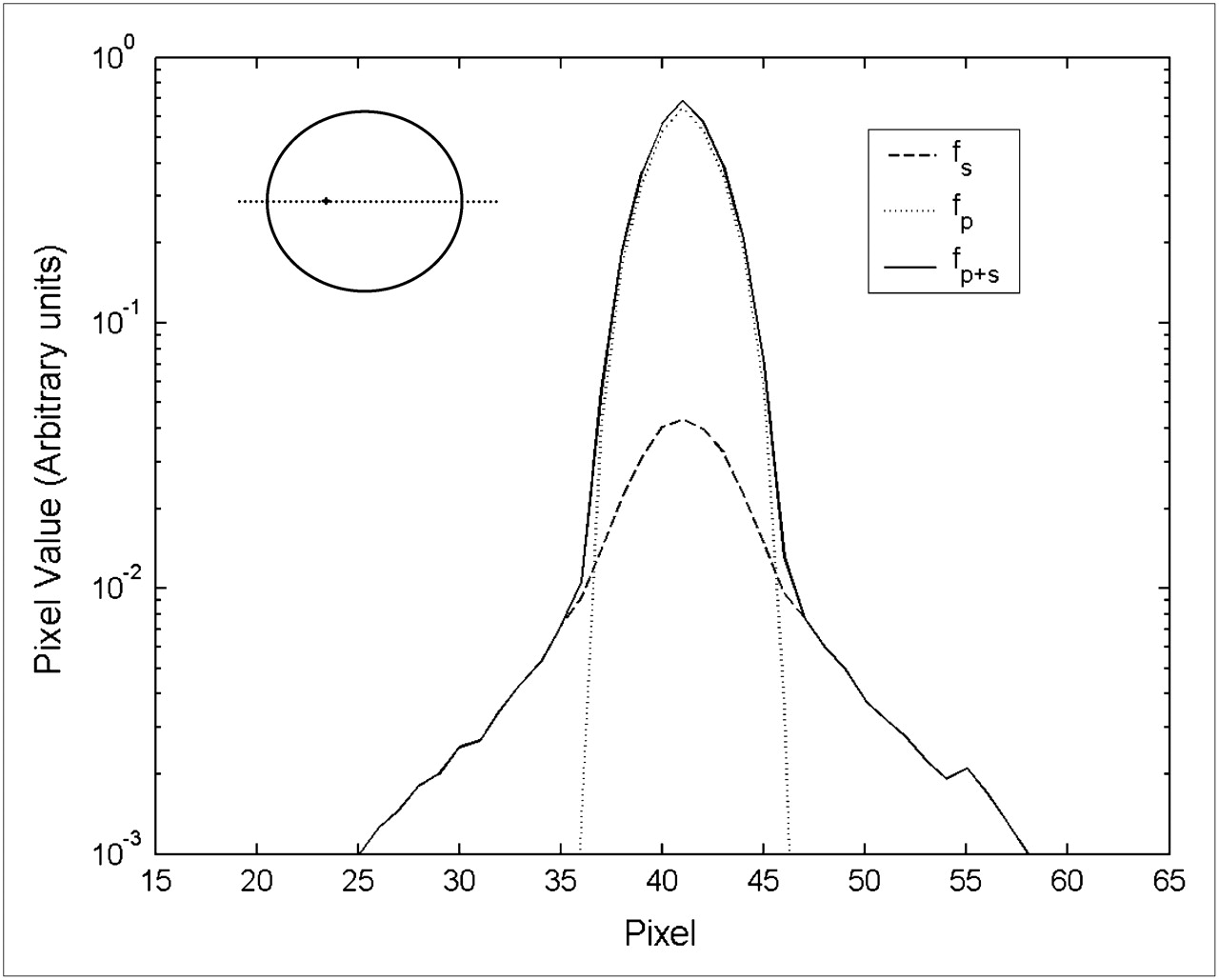
Monte Carlo simulations are performed to generate 2 sets of projection data: one is the primary scatter-free data, denoted by p; the other is the scattered data only, denoted by s. Then, we use fp and fs to represent the raw reconstructed images from primary and scattered photons, respectively. The sum of these 2 images (denoted by fp + s) is the raw image. To estimate the 2D PSF h defined in Equation 1, we generate a unit point source as the true image, and then the raw image fp + s becomes the 2D PSF for this specific source. The amplitude of the 2D PSF is determined by the total volume change in the image fp + s with respect to the image fp. To compare the scatter and collimator blurring parts in this 2D PSF, Fig. 1A shows the profiles of the images fp, fs, and fp + s reconstructed from a point source. The scattered photon image fs, compared with the primary photon image fp, contributes little to the width of the raw image fp + s. The scattering affects the 2D PSF by adding some volume and extended tails.

Profile of raw images along major axis in logarithmic scale.
Acknowledgments
This work was partially supported by NIH 5R21 EB006830 and by the Ben B. and Iris M. Margolis Foundation and the Benning Society. We thank Dr. Roy Rowley for his assistance with English editing.
Footnotes
-
COPYRIGHT © 2009 by the Society of Nuclear Medicine, Inc.
References
- Received for publication December 10, 2008.
- Accepted for publication March 4, 2009.


