


Abstract
In the present paper, a 2-dimensional adaptive autoregressive filter is proposed for noise reduction in images degraded with Poisson noise. In autoregressive models, each value of an image is regressed on its neighborhood pixel values, called the prediction region. The autoregressive models are linear prediction models that split an image into 2 additive components, a predictable image and a prediction error image. Methods: In this research, unfiltered images were split into smaller blocks, and best combinations of a prediction region and a block size for the image quality of predictable images were sought by using 3 Poisson noise–corrupted images with different image statistics. The images had dimensions of 128 × 128 pixels. Image quality was assessed by means of the mean squared error of the image. The adaptive autoregressive model was fitted into each block separately. Different degrees of overlapping of the image blocks were tested, and for each pixel the mean predictor coefficient of the different models was determined. The prediction error image was calculated for the entire image, and the filtered image was obtained by subtracting the prediction error image from the original image. The effect of the best adaptive autoregressive filter was illustrated using real scintigraphic data. Results: Generally, a prediction region of 4 orthogonal neighbors of the predicted pixel with a block size of 5 × 5 showed the best results. The use of 75% overlapping of the image blocks and 1 iteration of the filtering was found to improve prediction accuracy. The results were further improved when the 2 error term images were summed and subjected to adaptive autoregressive filtering and the resulting predictable image was added to the iteratively filtered image, allowing both noise reduction and edge preservation. Patient data illustrated effective noise reduction. Conclusion: The proposed method provided a convenient way to reduce Poisson noise in scintigraphic images on a pixel-by-pixel basis.
Autoregressive modeling uses past values of a 1-dimensional signal (1) or neighborhood values of a 2-dimensional signal (2) to extract important information from a signal. The number of past or neighborhood values used is called the model order. A 2-dimensional autoregressive model can be regarded as a low-pass filter that divides the image into 2 additive components, a predictable image and a prediction error image. Ideally, the prediction errors in a prediction error image should obey gaussian noise. The counting statistics in a scintigraphic image obey Poisson distribution, but with a mean value greater than, say 20, the counting statistics can be approximated by gaussian distribution (3). Therefore, 2-dimensional autoregressive models are, in theory, suitable for noise reduction in scintigraphic images. In the present paper, a new 2-dimensional adaptive autoregressive model for filtering of scintigraphic images is introduced. The adaptive autoregressive filter was tested using an artificial organlike scintigraphic image (4) with 3 different image statistics, and illustrated with patient data.
MATERIALS AND METHODS
Simulations
A transaxial slice of a Zubal phantom (Fig.1) (4) having dimensions of 128 × 128 pixels and a depth of 1 byte was used to test the adaptive autoregressive models. The Zubal phantom was originally designed to simulate x-ray–based CT images. In the present paper, the artificial pixel values are referred to as counts. A slice of the phantom simulated the upper abdominal region. The tests were performed using 3 images with different image statistics. The total counts of the images were 28,705 (low level), 54,469 (intermediate level), and 108,938 (high level). The mean counts of the images were 1.75, 3.3, and 6.6, respectively, and the range of pixel values was 0–32, 0–63, and 0–126, respectively. A built-in MATLAB function (version 2008a, The MathWorks, Inc.) was used to add noise to the images.
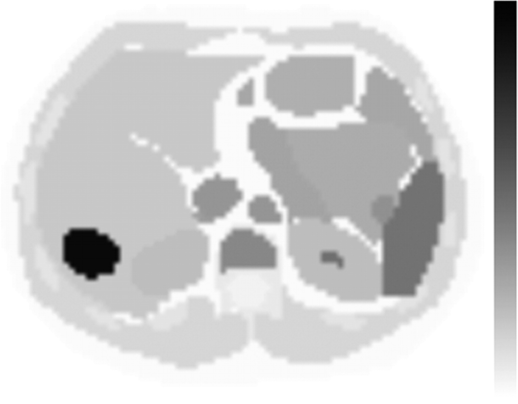
Slice of Zubal phantom. Inverse linear gray scale is used for comparison with original phantom.
Patient Data
Skeletal SPECT was performed 3 h after an intravenous injection of 555 MBq of 99mTc-labeled hydroxymethylene diphosphonate. The acquisition involved 64 stops at 30 s per stop and a 128 × 128 matrix. The range of pixel values was 0–84. The SPECT images were reconstructed by an iterative reconstruction technique (HOSEM Iterative Reconstruction, version 3.5; Nuclear Diagnostics). The number of subsets was set to 1 and the number of iterations to 10.
Autoregressive Model
In 2-dimensional autoregressive modeling, each value of an image is regressed on its neighborhood pixel values, called the prediction region (2). An autoregressive process x(n1,n2) is defined by
Multiplying both sides of Equation 1 by
This kind of linear set of equations is called a normal equation, and the solution results in a least squares estimate of the prediction coefficients a(n1,n2).
Suppose the data
As an example, a 5 × 5 pixel region of data is presented in Figure 2. The hatched area is the filter mask shape used, and the predicted sample is in the middle of the mask. Using Equation 1, we can write an estimate for every data point, as in the case of a 1-dimensional autoregressive model. Let the coordinates in the upper left corner be (n1,n2) = (0,0), that is, x(0,0) = 83, x(1,0) = 102, etc. Then

Support region (hatched area) of 2-dimensional autoregressive model. Current predicted pixel (gray area) is in middle of region.
The Equations 5 may be written in matrix form:
Adaptive Autoregressive Model
In a typical scintigraphic image, there are large local spatial variations in the count number of an image. This factor should be considered when one is using an autoregressive model for noise reduction in an image; that is, the same model cannot be applied to the entire image. In the present method, the image area was divided into smaller blocks, and the adaptive autoregressive model was then fitted into each block separately using MATLAB subroutines. Both forward and backward models were fitted into each block. Each block was first scanned from left to right and top to bottom and then backward. The predictor coefficients were calculated using the least squares minimization technique. Overlapping blocks were used, and for each pixel the mean predictor coefficient of the different models was calculated. The prediction error image was calculated for the entire image, and the filtered image was obtained by subtracting the prediction error image from the original image.
Assessment of Noise Reduction
The filtered image was subtracted from the phantom image, and the signal-to-noise ratio was estimated using the mean squared error. The mean squared error was calculated for different combinations of prediction region and block size. The prediction regions were 4 orthogonal neighbors of the predicted pixel, and 3 × 3 and 5 × 5 pixels. The block sizes were 4 × 4, 5 × 5, 6 × 6, 7 × 7, 8 × 8, 9 × 9, 10 × 10, 11 × 11, and 12 × 12 pixels. The effect of 50% and 75% block overlap, and the effect of iterative adaptive autoregressive filtering on the noise level, were tested. Finally, we checked whether the prediction error image contained important information that could be returned to the adaptive autoregressive filtered image. The best adaptive autoregressive filters were then compared with a 3 × 3 mean filter (convolution kernel: [1 2 1; 2 4 2; 1 2 1]/16) and a 3 × 3 median filter.
RESULTS
Simulations
When 50% overlap was used, a prediction region of 3 × 3 pixels with a block size of 7 × 7 performed best (Table 1). Noise reduction was better when 75% overlap was used. Again, the prediction region of 3 × 3 pixels displayed the best performance, but the best block size varied from 5 × 5 to 7 × 7 (Table 2).
Mean Squared Errors for Different Combinations of Prediction Region and Block Size When Degree of Overlap Is 50%
Mean Squared Errors for Different Combinations of Prediction Region and Block Size When Degree of Overlap Is 75%
The results improved after 1 iteration of adaptive autoregressive filtering, but 2 iterations decreased image quality (Table 3). At high and intermediate count levels, the prediction region of 3 × 3 pixels with a block size of 6 × 6 exhibited the best noise reduction. At a low count level, there were only minor differences between the different combinations.
Effect of Iteration on Mean Squared Errors for Different Combinations of Prediction Region and Block Size
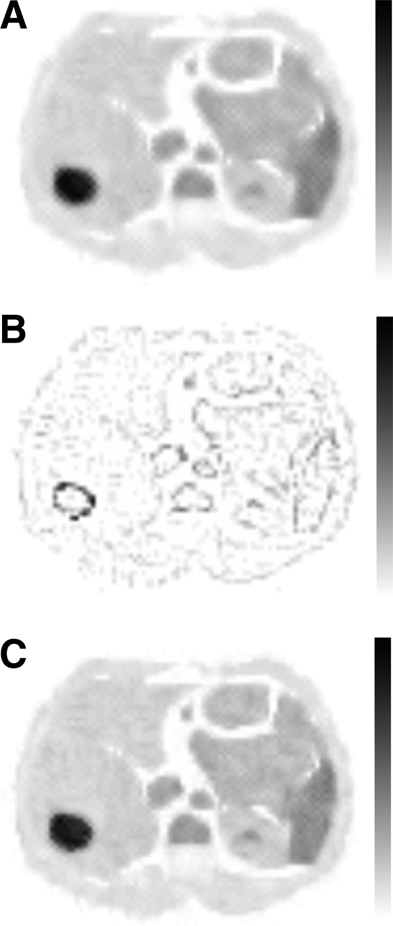
A further improvement in the results was achieved when the error term images were summed and subjected to adaptive autoregressive filtering and the resulting predictable image was added to the filtered image (Table 4; Fig. 3). The filtered error term images contained important information on the edges of the images. The prediction region of 4 orthogonal neighbors of a predicted pixel with a block size of 5 × 5 pixels performed best overall. Edge preservation was seen in the small areas with low counts (Fig. 4), as was confirmed by the profile analysis (Fig. 5). The adaptive autoregressive filter performed better than the conventional 3 × 3 mean filter (Table 5). The adaptive autoregressive filter was as efficient as the 3 × 3 median filter at low and intermediate count levels but not at a high count level. However, the image produced by the adaptive autoregressive filter at a high count level was visually closer to the phantom image than that produced by the median filter (Figs. 4 and 6), especially in the small areas with no counts or low counts.
Effect of Adding Filtered Error Term Image to Predictable Image
Total Counts and Mean Squared Errors of Poisson Noise–Corrupted Images and Images After Removal of Noise Using Best Adaptive Autoregressive Model, 3 × 3 Mean Filter, and 3 × 3 Median Filter

Iteratively filtered image (A) summed with filtered error term image (B) to get final image (C). Images are individually scaled to their own maximum. Count level is intermediate.

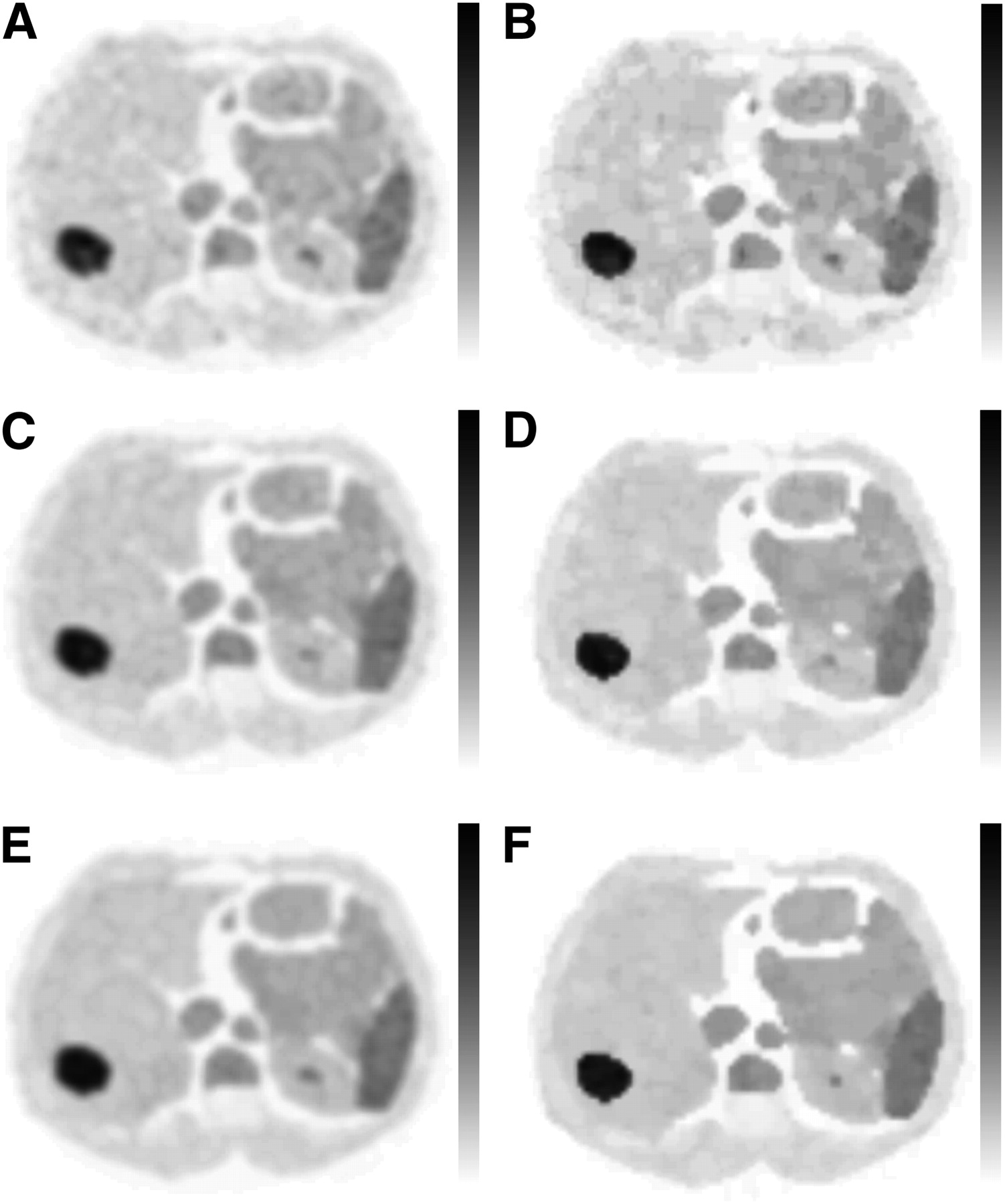
Low- (A), intermediate- (C), and high-count (E) phantom images corrupted by Poisson noise. Noise was removed using best adaptive autoregressive model (B, D, and F). Images are individually scaled to their own maximum.

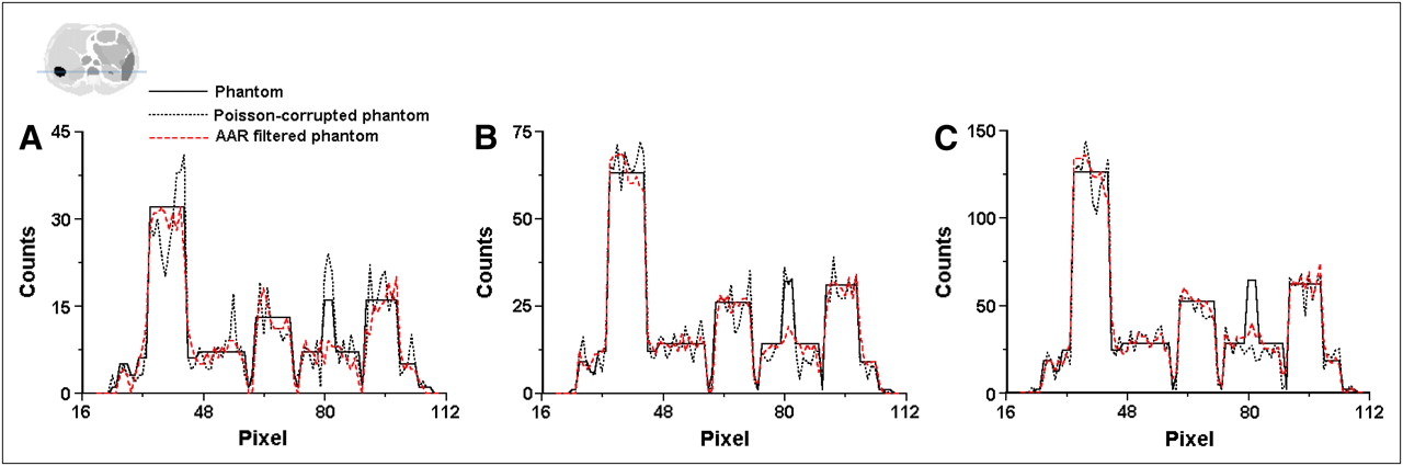
One-pixel-thick profile curves drawn through Zubal phantoms, noise-corrupted Zubal phantoms, and phantoms filtered using best adaptive autoregressive model, at level shown by phantom. Count levels are low (A), intermediate (B), and high (C). AAR = adaptive autoregressive model.

Low-, intermediate-, and high-count phantom images filtered with 3 × 3 mean filter (A, C, and E) and 3 × 3 median filter (B, D, and F). Images are individually scaled to their own maximum.
Patient Data
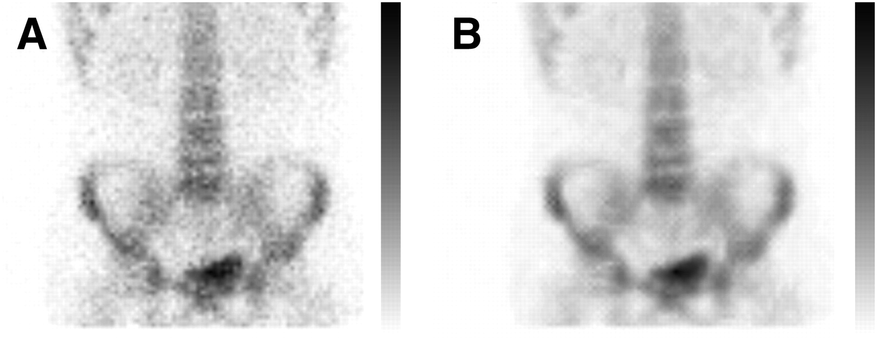
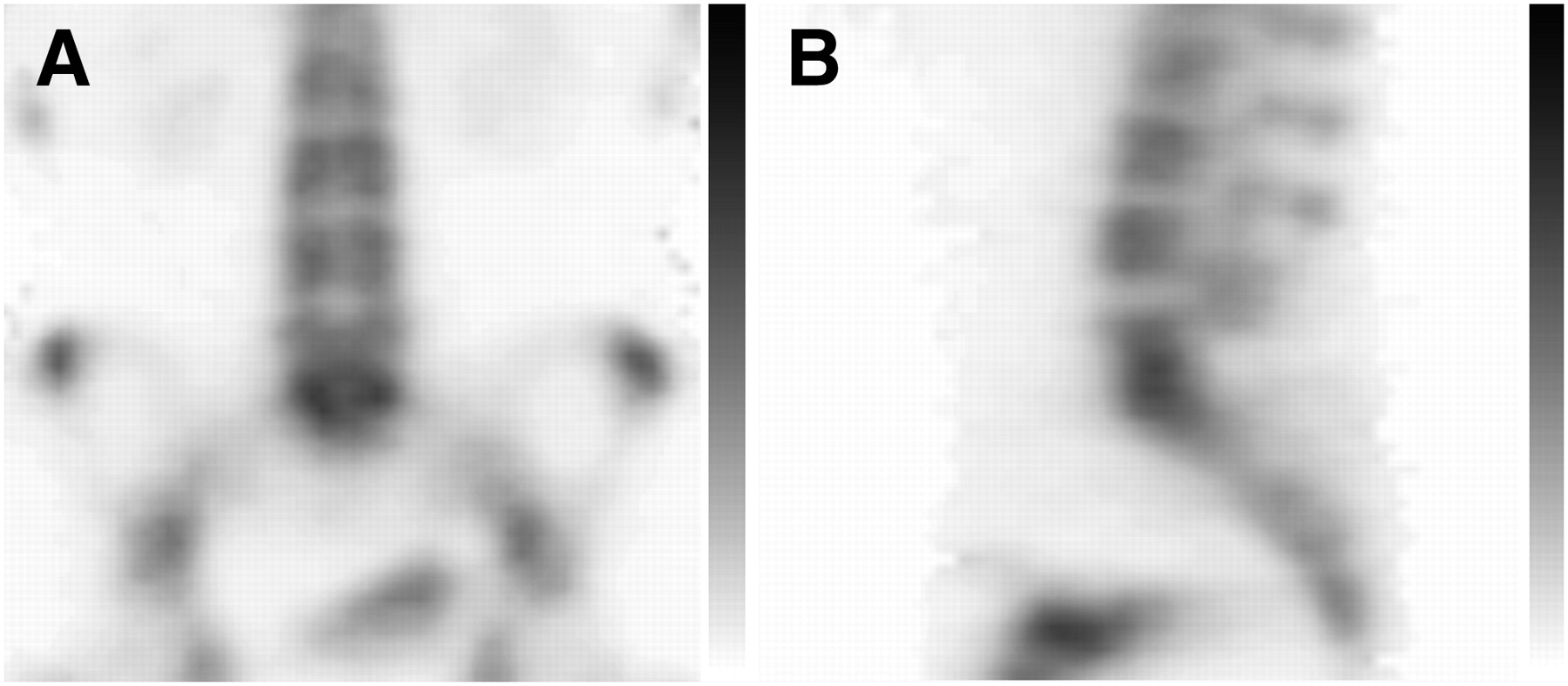
Figure 7 shows projection image data in the skeletal SPECT study before and after adaptive autoregressive filtering, and the effect of adaptive autoregressive filtering on tomographic slices is illustrated in Figure 8.

Noisy projection image of skeletal SPECT (A), and projection image with noise removed (B). Adaptive autoregressive model is used, with prediction region of 4 orthogonal neighbors of predicted pixel and block size of 5 × 5 pixels.

Adaptive autoregressive filter was applied to projection data, and transversal slices were reconstructed with iterative method. Shown are reformatted coronal (A) and sagittal (B) slices of skeletal SPECT image. Adaptive autoregressive model is used, with prediction region of 4 orthogonal neighbors of predicted pixel and block size of 5 × 5 pixels. No additional noise removal methods were applied.
DISCUSSION
In the present paper, we have proposed a new filter for reducing Poisson noise in scintigraphic images. It is based on a classic autoregressive model. The novel ideas were to apply iterations on a planar image, to use a spatially varying (i.e., adaptive) autoregressive model, and to use information on the error term images for edge restoration. Our filter is suited to removing the noise from scintigraphic planar images or projection images of a SPECT study.
In medical imaging, different 2-dimensional autoregressive models have thus far been used for lossless image compression (5,6) and texture characterization (7) but, to our knowledge, not for noise removal from scintigraphic images.
The Poisson-corrupted torso images we used to test our new filter actually represented artificial scintigraphic planar images. We used 3 Poisson-corrupted artificial scintigraphic images with different image statistics. Image quality was best when a 75% overlap of the image blocks in combination with 1 iteration of the filtering procedure was used. Importantly, we found that the error term image contained important information about the edges of the image. Part of the counts at the edges could be returned to the filtered image, reducing blurring of the image but at the cost of some increase in the noise. The best results were achieved with the smallest possible symmetric prediction region, that is, 4 orthogonal neighbors of the predicted pixel, with a block size of 5 × 5 pixels. This method provided good noise reduction while maintaining high resolution and had the best edge preservation property.
In medical imaging, scintigraphic images are inherently noisy, and there are large local spatial variations in the count number of the images. Because our new filter works in the spatial domain, its characteristics can be adapted to match the nature of the data on a pixel-by-pixel basis—something that is not possible when filtering is done in the frequency domain. The computational time is longer in spatial domain filtering than in traditional filtering in the frequency domain, but because of fast computers, that factor is no longer important in clinical praxis. An additional advantage of the adaptive autoregressive filter is that it does not need any parameters. Therefore, it might be an all-purpose filter in the future.
The quality of planar images can be improved using contrast-enhancing and noise-reducing filters, which can increase both the sensitivity and the specificity of a study (8). However, filtering is essential especially in image reconstruction of SPECT studies, because emission tomography acquisition data are subject to substantial statistical noise. Filtering can be performed before reconstruction (filtering of projections, prefiltering), during reconstruction, or after reconstruction (postfiltering).
Until recently, filtered backprojection has remained the most frequently used reconstruction technique in nuclear medicine (9,10). In traditional filtered backprojection, filtering is performed both before reconstruction through the application of a low-pass filter on projection images and during reconstruction through the application of a ramp filter. Prefiltering should be applied, because a ramp filter amplifies high frequencies.
Filtered backprojection is not the only way to reconstruct from projections, but since 1970 (11) there have been various iterative (algebraic) reconstruction methods available. Iteration is a repeated calculation process in which the algorithm uses all the projection data several times in attempting to yield successively better approximations of the spatial distribution of the tracer in the tissue. A common problem with iterative algorithms is the increase of noise in the reconstructed image when the number of iterations increases. On the other hand, too early termination of iterations can result in a biased image (12). In iterative methods, filtering is typically done during reconstruction. Sometimes, postfiltering is applied in iteratively reconstructed images.
Our new filter can be applied to the projection data independently of the reconstruction method and, in the future, might be a complementary aid in advanced iterative reconstruction techniques.
A limitation of our filter is that it cannot take into account the Poisson image statistics. Scintigraphic data follow Poisson distribution. Unlike gaussian distribution, this is a long-tailed distribution. However, Poisson distribution can be approximated by a gaussian distribution for a mean intensity roughly greater than 20. This is not always true in practice, but locally varying filters, such as our filter, have been shown to effectively reduce Poisson-type noise in low-count images (13,14).
CONCLUSION
A new theoretic way to reduce noise in scintigraphic images was introduced. The presented filter reduces noise in scintigraphic images in a natural manner.
REFERENCES
- Received for publication March 9, 2010.
- Accepted for publication October 18, 2010.


Jump to section
Related Articles
Cited By...
- No citing articles found.