This Article Abstract Figures Only Full Text (PDF) CME Activity Supplemental Data Alert me when this article is cited Alert me if a correction is posted Services Email this article to a friend Similar articles in this journal Similar articles in PubMed Alert me to new issues of the journal Download to citation manager Citing Articles Citing Articles via HighWire Citing Articles via Google Scholar Google Scholar Articles by Goldman, L. W. Search for Related Content PubMed PubMed Citation Articles by Goldman, L. W.

Principles of CT and CT Technology^*

Department of Radiation Therapy and Medical Physics, Hartford Hospital, Hartford, Connecticut

Correspondence: For correspondence or reprints contact: Lee W. Goldman, Department of Radiation Therapy and Medical Physics, Hartford Hospital, 80 Seymour St., Hartford CT 06102. E-mail: lgoldma{at}harthosp.org

ABSTRACT

This article provides a review of the basic principles of CT within the context of the evolution of CT. Modern CT technology can be understood as a natural progression of improvements and innovations in response to both engineering problems and clinical requirements. Detailed discussions of multislice CT, CT image quality evaluation, and radiation doses in CT will be presented in upcoming articles in this series.

Key Words: CT; CT technology; imaging; reconstruction

The use of CT in nuclear medicine imaging has been growing, first with the introduction of PET combined with CT (PET/CT) and, more recently, with the introduction SPECT combined with CT (SPECT/CT). In addition, some of the basic ideas underlying CT, such as reconstruction from projections (i.e., data measured at many positions and angles), are very similar to those underlying the nuclear medicine cross-sectional imaging modalities PET and SPECT. This article is the first of 3 to deal with the principles of CT and CT technology. This first article covers the fundamental principles of CT, including the basic geometry of the CT scan process, the nature of the measurements made by CT detectors, a qualitative explanation of the image reconstruction process, the evolution of CT technology (the 4 generations of CT) from the EMI first-generation scanner through modern slip ring designs, and the process of helical CT. The next 2 articles will cover image quality and radiation doses in CT and multislice CT.

LIMITATIONS OF CONVENTIONAL RADIOGRAPHY

Film/screen radiography has several drawbacks that limit its ability to visualize low-contrast tissues and structures with acceptable levels of patient radiation exposure. These limitations include the following.

Inefficient x-Ray Absorption
Before the introduction of rare earth–intensifying screens 20–25 y ago, the x-ray absorption efficiency of typical par-speed/calcium tungstate film/screen cassettes was only about 25%. Thus, 75% of the available x-ray beam as well as 75% of the information was wasted.

High Scatter–to–Primary x-Ray Ratios
Because of large beam areas, scattered photons represented 50% or more of the x-rays absorbed by the screens, even with a grid able to remove high levels of scatter. Scatter effectively reduces subject contrast by creating a background intensity unrelated to the overlying anatomy. The amount of lost subject contrast is given by the contrast reduction factor, 1/[1 + (S/P)], where S and P are the scatter and the primary x-ray intensities at the receptor, respectively (1). If 50% of the detected x-rays are scatter (so that S = P), then subject contrast is reduced by a contrast reduction factor of 0.5.

Superimposition and Conspicuity
Conspicuity is the ease of finding an image feature during a visual search. A feature may be visible if one knows where to look but may be missed—that is, it may be inconspicuous—if the image is complex. Radiography renders a 3-dimensional volume onto a 2-dimensional image; as a consequence, over- and underlying tissues and structures are superimposed, generally resulting in reduced conspicuity as well as subject contrast.

Receptor Contrast Versus Latitude
Clinically useful radiographic films must provide sufficient exposure latitude (i.e., a range of exposures yielding clinically acceptable film densities) to record as much of the range of x-ray intensities exiting the patient as possible; this feature necessarily limits receptor contrast. For example, for a typical radiographic film with an average gradient (i.e., film contrast) of 2.5, an intensity (I) difference of 1.0% would yield a film optical density (OD) difference of

and (in the usual absence of well-defined edges) would not be visible.

Although improved x-ray absorption efficiency is available with modern radiographic technology and digital radiography has nearly eliminated the contrast–latitude trade-off, most of these limitations of radiography still exist today.

These issues were recognized long before the development of CT, which led investigators to consider improvements. One such innovation was conventional (focal-plane) tomography, described by Bocage (2) in 1921. Through simultaneous movement of the x-ray tube and the receptor around a fulcrum, tomography improved conspicuity by blurring over- and underlying structures.

Both conspicuity and contrast could be improved if irradiation and visualization were limited to individual cross-sectional imaged slices, which could be displayed as 2-dimensional images without significant structure overlap. Because the radiation source could be collimated to thin (1-cm) slices, significantly less scatter would be generated (because less tissue would be irradiated at any given time) as well. One way to achieve this goal is the process of reconstruction from projections. Interestingly, the theory of image reconstruction from projections, which is central to the basic concept of CT, was described in 1917 and was proposed for medical imaging as early as 1940 (3).

The development of the first modern CT scanner was begun in 1967 by Godfrey Hounsfield, an engineer at British EMI Corp. Hounsfield was interested in situations in which large amounts of potential information may be inefficiently used—an accurate description of conventional radiography for the reasons cited earlier (4,5). He estimated that by taking careful measurements of x-ray transmission through a subject at many positions across the subject and at a sufficient number of angles, it should be possible to determine attenuation differences of 0.5%—possibly sufficient to distinguish between soft tissues. After verification of his hypothesis with a laboratory apparatus, the first clinical CT scanner was built and installed at Atkinson-Morley Hospital in England in September 1971. To understand the basic principles of CT, one may begin with the operation of this original EMI Mark I first-generation CT scanner.

BASIC PRINCIPLES OF CT: FIRST GENERATION OF CT

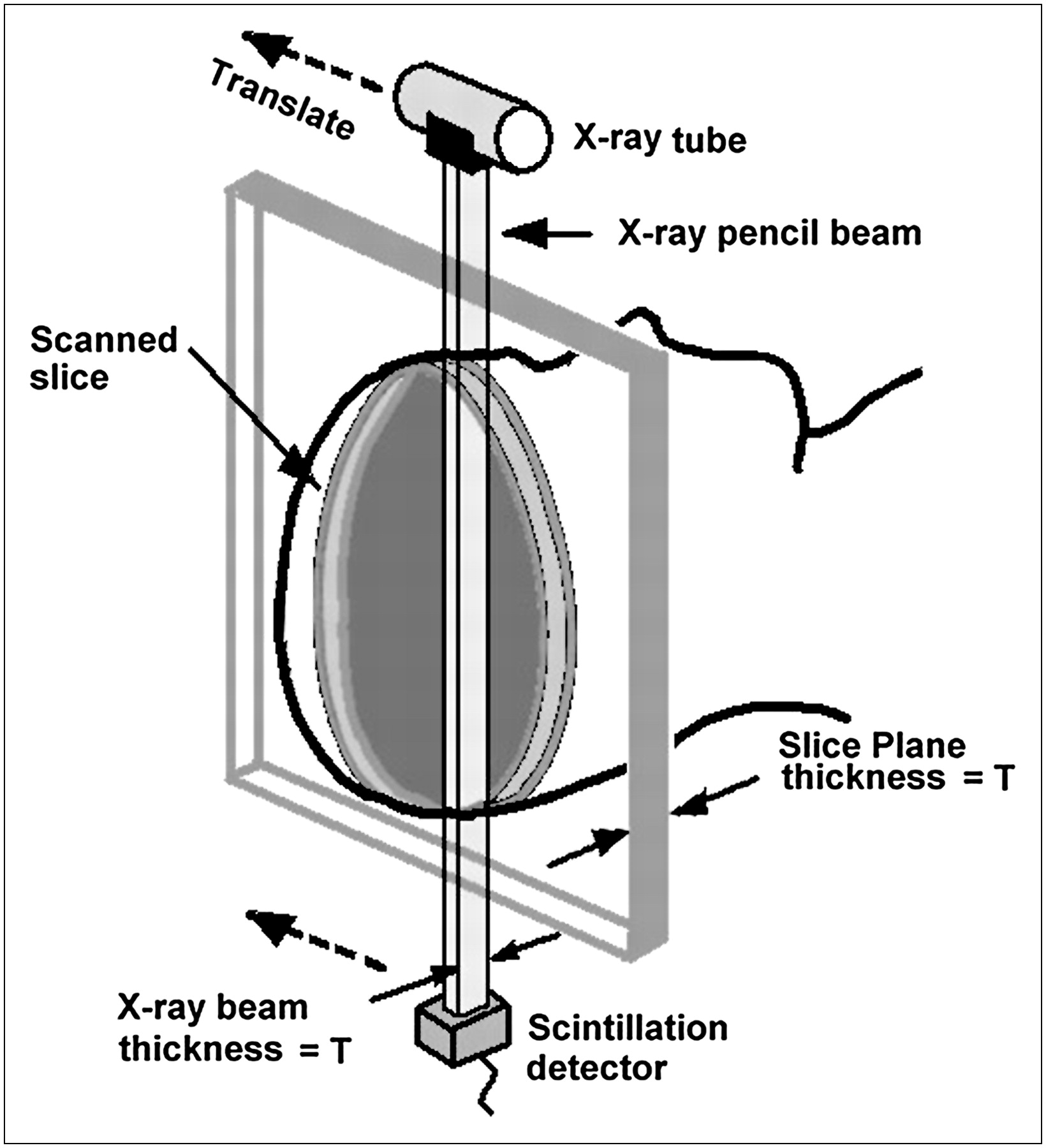
Hounsfield imagined the subject to be scanned as being divided into axial slices. The x-ray beam to be used was collimated down to a narrow (pencil-width) beam of x-rays. The size of the beam was 3 mm within the plane of the slice and 13 mm wide perpendicular to the slice (along the axis of the subject). In fact, it is this beam width that typically specifies the slice thickness to be imaged. The x-ray tube is rigidly linked to an x-ray detector located on the other side of the subject. Together, the tube and the detector scan across the subject, sweeping the narrow x-ray beam through the slice (6). This linear transverse scanning motion of the tube and the detector across the subject is referred to as a translation. The arrangement is diagramed in Figure 1.

View larger version (37K): [in this window] [in a new window]   FIGURE 1.  CT arrangement. Axial slice through patient is swept out by narrow (pencil-width) x-ray beam as linked x-ray tube–detector apparatus scans across patient in linear translation. Translations are repeated at many angles. Thickness of narrow beam is equivalent to slice thickness.

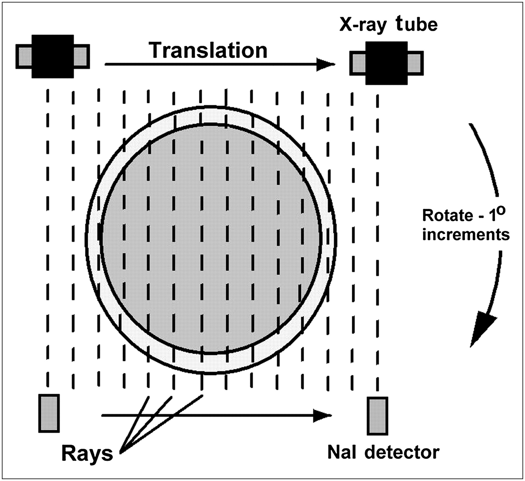
View larger version (38K): [in this window] [in a new window]   FIGURE 2.  x-Ray transmission measurements. Measurements are obtained at many points during translation motion of tube and detector. x-Ray path corresponding to each measurement is designated a ray, and set of rays measured during translation is designated a view. Views are collected at many angles (in 1° increments in this example) to acquire sufficient data for image reconstruction.

CT IMAGE RECONSTRUCTION

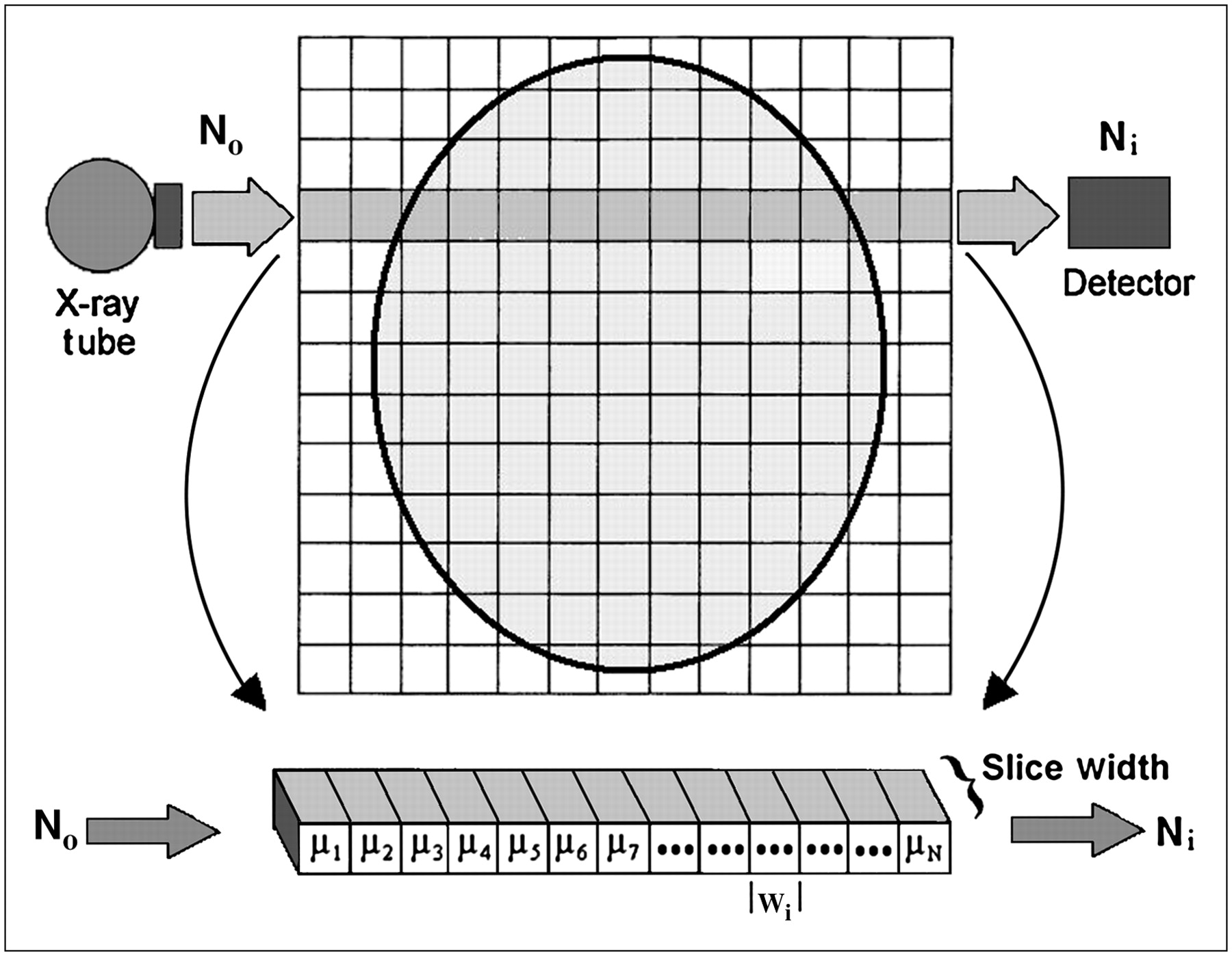
Hounsfield envisioned dividing a slice into a matrix of 3-dimensional rectangular boxes (voxels) of material (tissue) (Fig. 3). Conventionally, the X and Y directions are within the plane of the slice, whereas the Z direction is along the axis of the subject (slice thickness direction). The Z dimension of the voxels corresponds to the slice thickness. The X and Y voxel dimensions ("W" in Fig. 3) depend on the size of the area over which the x-ray measurements are obtained (the scan circle) as well as on the size of the matrix (the number of rows and columns) into which the slice is imagined to be divided. For example, suppose that each translation covers 250 mm. After collection of all of the views, the measurements cover a scan circle with a diameter of 250 mm. If this scan circle is divided into a matrix of 250 rows x 250 columns, each voxel is 1 x 1 mm. If a 512 x 512 matrix is used (as is common today), each voxel is approximately 0.5 x 0.5 mm. This matrix is referred to as the reconstruction matrix.

View larger version (49K): [in this window] [in a new window]   FIGURE 3.  Reconstruction matrix. Hounsfield envisioned scanned slice as being composed of matrix of small boxes of tissue called voxels, each with attenuation coefficient µ. x-Ray transmission measurements (Ni) can be expressed as sum of attenuation values occurring in voxels along path of ray for Ni.

To carry out reconstruction, consider the row of voxels through which a particular ray passes during data collection (bottom of Fig. 3). N_i is the transmitted x-ray intensity for this ray measured by the detector. N_o is the x-ray intensity entering the subject (patient) for this ray. It can be shown (Appendix) that a derived measurement X_i can be related to a simple sum of the attenuation values in the voxels along the path of the ray; for the row of voxels in Figure 3, this relationship is

(Eq. 1)

where X_i = –ln(N_i/N_o) and u_i =w_iµ_i is the attenuation of voxel i. Similarly, measurements for all rays at all positions and angles can be expressed as sums of the attenuation values in voxels through which each ray has passed. Note that the quantity X_i is known; it is calculated from each detector measurement N_i with the known X and Y voxel dimensions (W) and the known x-ray intensity entering the patient (N_o). In Hounsfield's scanner, N_o was directly measured by a reference detector sampling the x-ray intensity exiting the x-ray tube. Modern scanners determine N_o from routine calibration scans.

For example, consider a simple 2-row by 2-column reconstruction matrix (Fig. 4A). Views are collected at 4 angles, 0° (left to right), 90° (top to bottom), 45° (diagonal), and 135° (diagonal), and each measurement is expressed as the sum of the voxel attenuation values along each ray. In this case, there are 6 equations:

and

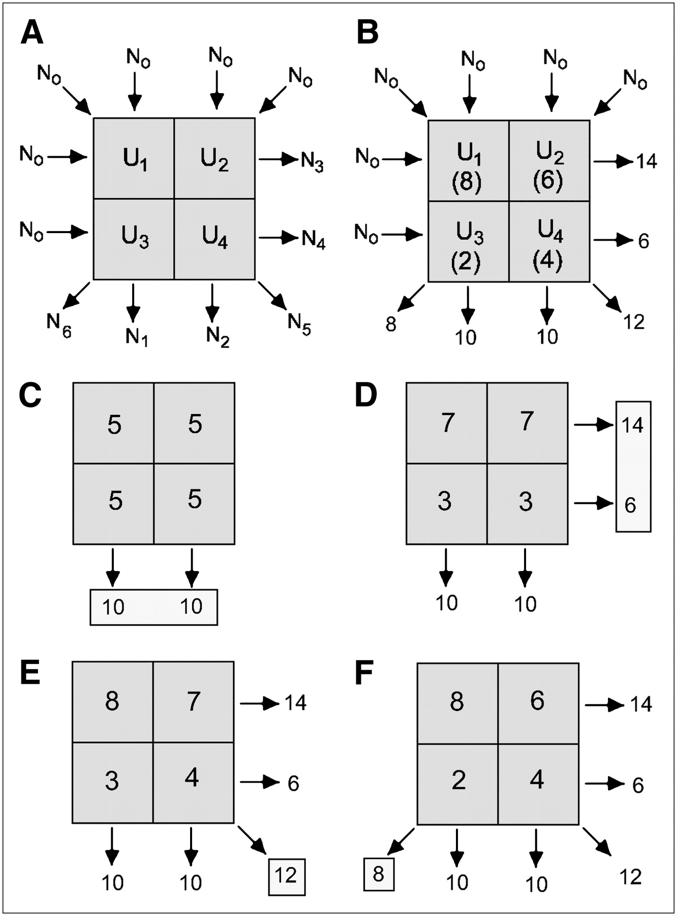
View larger version (26K): [in this window] [in a new window]   FIGURE 4.  ART. (A) ART algorithm for 4-voxel "patient." (B) Attenuation measurements. (C) Starting estimate is constructed by dividing measurements from first view equally along their ray paths. (D–F) This estimate is iteratively adjusted to match measurements for each consecutive view, stopping when transmission measurements predicted by current estimate match all actual measurements to within some preset tolerance.

and

Next, these adjustments are divided equally along the rays, adding 2 to u₁ and u₃ (total adjustment of +4) and subtracting 2 from u₂ and u₄ (total adjustment of –4), yielding the second estimate (Fig. 4D). The process continues in this manner, with the actual values for each view being compared in turn with the values predicted by the latest estimate. For the third view (measurement 5), the second estimate predicted an attenuation value of 10 (7 + 3); the actual value was 12. Thus, the +2 total adjustment is divided equally along the ray for X₅', subtracting 1 each from u₁ and u₄, to generate the third estimate (Fig. 4E). The required adjustment for the fourth view (a total of –2) is divided along the ray (subtracting –1 from u₂ and u₃) to generate the fourth and last estimate (Fig. 4F). Because the attenuation values predicted by this last estimate match all actual measurements, the image is accepted as the true reconstructed image (and one can see that it matches the parenthetical values in Fig. 4B).

ART images were typically available within 20 s of scan completion. In practice, however, ART was sensitive to quantum noise and could result in poor image quality if transmitted x-ray intensities were low. As in conventional radiography, noise (graininess) in CT images arises from a limited number of x-ray photons contributing to each measurement (because a limited patient radiation dose is used). This noise, known as quantum mottle, appears as unavoidable random fluctuations (random errors) in detector measurements and is described by the Poisson statistical distribution. The magnitude of the fluctuations is given by the square root of the number of photons contributing to the measurements. For example, if 100 x-rays were included in measurement X₃ in Figure 4B, then the size of the fluctuations (noise) would be the square root of 100, or 10. If repeated measurements of X₃ were obtained for the same subject with the same apparatus, then the measurements would randomly fluctuate around an average of 100, with approximately two thirds of the trials being between 90 and 110 (i.e., 100 ± 10).

The problem with ART can now be explained: No estimate that ART generates will ever match all measurements exactly, because the measurements include random errors. Thus, ART must be discontinued after an estimate that matches all measurements only within some tolerance is found; for high noise (low intensities), that tolerance may not be met even after many iterations. Fortunately, the early success of CT created a wealth of research and development activities (discussed later). One such innovation was a much better reconstruction algorithm based on the idea of backprojection.

Backprojection is illustrated in Figure 5. Suppose that a simple test object containing 3 objects with different attenuation values is scanned as shown in Figure 5A and that views (attenuation measurements) are obtained at 3 angles. For each view at each angle, the reconstruction process is very straightforward. The attenuation measurements of each view are simply divided evenly along the path of the ray; this process is called backprojection. An example of backprojection for the view measured at 0° is shown in Figure 5B. Note that after backprojection of only 4 views, an image of the test object is beginning to appear in Figure 5C.

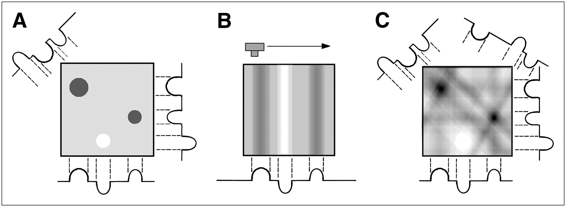
View larger version (18K): [in this window] [in a new window]   FIGURE 5.  (A) Backprojection reconstruction for simple phantom containing 3 objects with different attenuation values. (B) For each view, attenuation values are simply divided evenly along their ray paths. Summing backprojected views from several angles builds image. (C) Four views of phantom are summed. Although this method is efficient, images reconstructed with backprojection exhibit considerable blurriness.

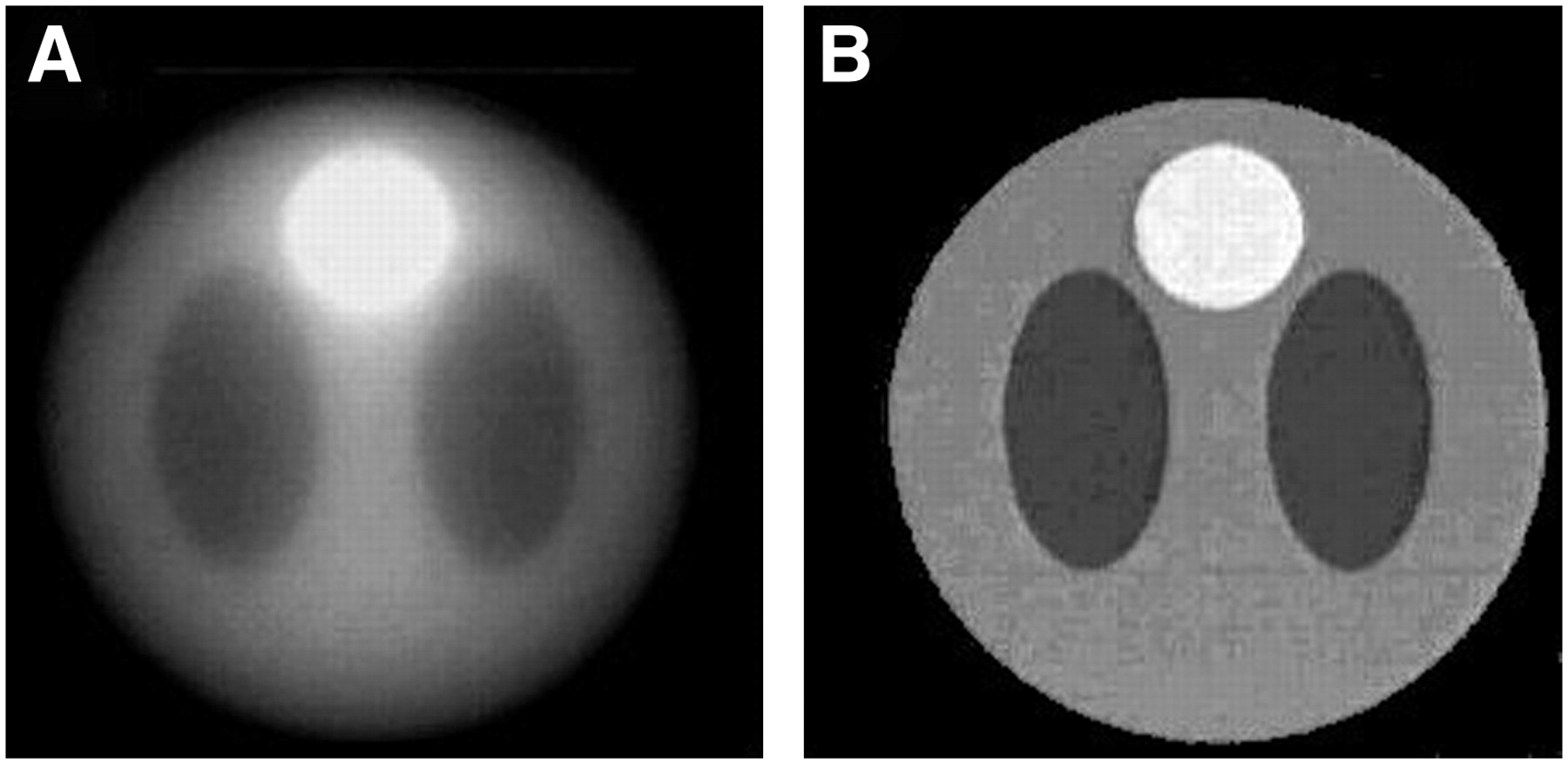
View larger version (55K): [in this window] [in a new window]   FIGURE 6.  FBP. Mathematic phantom image reconstructed without (A) and with (B) filtering. FBP effectively reconstructs high-quality images. Adapted from S. Napel.

CT IMAGE PRESENTATION

A convention that has existed from the earliest days of CT is to replace the attenuation value calculated for each voxel of the reconstruction matrix with an integer (CT number) calculated as follows:

(Eq. 2)

In this equation, u_voxel is the calculated voxel attenuation coefficient, u_water is the attenuation coefficient of water, and K is an integer constant. In the original EMI scanner, K was 500, but K later become standardized as 1,000 (or sometimes 1,024). The reason for calculating CT numbers relative to water is discussed in the next section. Scanners today determine u_water from periodic calibration scans of water or water-equivalent phantoms. Because attenuation coefficients are affected by x-ray beam energy, proper x-ray generator calibration is important for accurate and reproducible CT numbers. Note that the quantity is referred to as CT number, but the units are Hounsfield units (to honor the inventor). Thus, one would say, for example, that a particular tissue in an image "has a CT number of 40 Hounsfield units."

Some examples of CT number calculations are as follows: A voxel actually containing water would have a CT number of 0 (for a well-calibrated scanner), because u_water – u_water = 0 (the CT number of water will always be approximately 0 but not necessarily exactly 0 because of quantum mottle); if the voxel contained air (for which u_air 0), the CT number would be approximately –1,000; and for a voxel containing dense cortical bone (for which u 2 u_water), the CT number would be approximately +1,000.

Displaying the full possible CT number range (–500 to 500 for the original EMI scanner and –1,000 to +1,000 for scanners introduced soon after that) presents a problem: Even today, displays often show only about 250 shades of gray, of which fewer (perhaps as few as 100) may be visually discernible. If the full CT number range of 2,000 (–1,000 to +1,000) is spread evenly over 200 discernible gray levels, each level represents a range of 10 CT numbers. However, it can be seen from Equation 2 that a 0.5% attenuation difference—well within the ability of CT to distinguish—corresponds to a CT number difference of 5 Hounsfield units. Many soft-tissue structures would be displayed with the same gray level as their surroundings and thus would be invisible. In fact, a material must differ from its surroundings by at least 1% to ensure a different gray level. Tissues of most common interest in CT generally lie in the CT number range of –100 to +100 (7). If instead discernible gray levels were limited to the CT number range of –100 to +100, then no bone details (all white) and no lung details (all black) would be visible. The solution, which is taken for granted today, is windowing, illustrated in supplemental Figure 3. A viewer may (interactively) decide how gray levels are to be allocated by specifying a window width (the range of CT numbers to display, e.g., –50 to 200) and a window level (or window center, e.g., 0). Adjustable window settings may then be altered to view other CT number ranges. Universally today, windowing can be interactively performed with a mouse or trackball.

FIRST-GENERATION EMI CT SCANNER

The original EMI device was a dedicated head scanner in which the patient's head was recessed via a rubber membrane into a water-filled box (supplemental Figs. 4 and 5). The device was designed such that the water-filled box rotated (in 1° increments) along with the single-narrow-beam, single-detector assembly, resulting in a fixed path length through patient plus water for all rays and transmission measurements.

The results obtained with this first clinical EMI scanner (installed in September 1971) were presented at a British radiologic society meeting in April 1972. The results left no doubt as to the revolutionary clinical value of the process. The historic success of the scanner created enormous interest and led to an explosion of research and development by many groups and corporations. One such development was FBP reconstruction, described earlier. However, a technology race to improve and expand the CT process was also under way.

Of course, one important application was body scanning, but the water-filled box had to be eliminated. However, a discussion of why it was used in the first place is worthwhile. It served 2 purposes, both of which allowed Hounsfield to maximize the accuracy of attenuation coefficient measurements. These 2 reasons were as follows.

Limitation of Dynamic Range
The water-filled box greatly reduced the range of intensities over which the detector needed to accurately respond, thus allowing optimization of the detector sensitivity.

Beam-Hardening Correction
x-Rays produced in x-ray tubes are mostly bremsstrahlung x-rays which, unlike the discrete photon energies emitted by radioactive isotopes, cover a broad continuum of energies (up to a maximum numerically equal to the x-ray tube kilovoltage). Such beams are referred to as polychromatic. Beam hardening refers to a gradual increase in the effective energy of polychromatic x-ray beams as they penetrate deeper into attenuating materials. It is caused by preferential attenuation of the lower-energy (and thus less penetrating) photons in the beam by each successive layer of attenuating material (1). Because attenuation coefficients depend on both the material and beam energy, the same tissue at a greater depth has a lower attenuation coefficient (because the deeper tissue attenuates less of the hardened x-ray beam).

During scanning of a uniform object (e.g., a cylindric water-filled phantom), beam hardening causes lower attenuation coefficients to be reconstructed for deeper voxels, producing an undesired "cupping" artifact in which the same material appears darker in the center of the image than in the periphery. To understand how the water-filled box allowed Hounsfield to correct for this beam-hardening effect, consider the path of one of the measurements through the water-filled box and patient. As in Equation 1, the measurement is expressed as a sum of the attenuation coefficients of the voxels through which it passes:

Now consider a measurement made along an identical path length but passing only through water:

In fact, it is evident from supplemental Figure 5 that water-only measurements can be made at the beginning and end of every view, when the narrow beam passes outside the edges of the patient's head. Because each voxel along the path of X_w contains water, each voxel can be corrected for beam hardening (because all of the voxels must have the same attenuation coefficient—that of water). The next step is to subtract X_w from X_a:

(Eq. 3)

The attenuation coefficients of soft tissues differ by only a few percentage points from that of water. Therefore, the terms of Equation 3 represent small corrections for the attenuation coefficient of each voxel relative to that of water—the latter can be corrected (from the water-only path). By comparing each measurement with a water-only measurement, Hounsfield was actually calculating attenuations as u_i – u_w (rather than u_i), a factor that explains the numerator of Equation 2: CT numbers were calculated from u_i – u_w because those were the values that Hounsfield actually reconstructed.

To eliminate the water-filled box and expand the usefulness of CT, the functions that the box served must be replaced. In part, this goal is accomplished by use of a "bow-tie" filter through which the beam passes when exiting the x-ray tube. First, the filter (usually made of aluminum) is thicker where the path through the patient is shorter (toward the edges), effectively limiting the range of intensities reaching the detector. Second, the filter prehardens the beam (i.e., it removes the lower-energy x-rays), so that less hardening occurs in the patient. The remainder of the beam-hardening correction is done with software and periodically performed calibration scans of uniform phantoms of various sizes. Although quite sophisticated and effective, software beam-hardening corrections are only approximate, and nonuniformities can in fact often be observed in scans of uniform phantoms when a very narrow display window is used.

REDUCING SCAN TIME: SECOND GENERATION OF CT

The first waterless full-body CT scanner was developed and installed by Ledley et al. at Georgetown University in February 1974 (8). This device introduced several innovations now standard in CT (table movement through the gantry, gantry angulation, and a laser indicator to position slices) as well as a Fourier-based reconstruction algorithm mathematically equivalent to FBP (R.S. Ledley, personal communication) but still used first-generation design, with scan times of 5–6 min. As a result, body scans were unavoidably corrupted by patient motion.

A step toward reduced scan times was taken with the introduction of second-generation CT geometry in late 1974 (9). Second-generation CT used multiple narrow beams and multiple detectors and, as in the first generation, used rotate–translate motion. A second-generation scanner with 3 narrow beams and 3 detectors is shown in supplemental Figure 6 and diagramed in Figure 7 (the 3 photomultiplier tubes associated with the 3 detectors can be seen to the right of the patient aperture in the photograph in supplemental Fig. 6). It may seem at first that second-generation CT accelerated data collection via simultaneous measurements at each point along a translation. In fact, if the set of rays measured by each detector is considered (Figs. 7B–7D for the left, center, and right detectors, respectively), it can be seen that the detectors actually acquire their own separate, complete views at different angles. If there is a 1° angle between each of the 3 narrow beams, then one translation collects data for views at, for example, 30°, 31°, and 32°. Only one third as many translations are required, and scan time is reduced 3-fold; what took 6 min now takes 2 min. In general, second-generation CT can reduce scan time by a factor of 1/N, where N is the number of detectors.

View larger version (48K): [in this window] [in a new window]   FIGURE 7.  Second-generation data collection. (A) Transmissions of multiple narrow beams (3, in this case) were simultaneously acquired by multiple detectors during each translation. (B–D) Small angle between narrow beams allowed each detector to acquire complete separate view at different angle. Number of required translations was correspondingly reduced by factor of 1/(number of detectors).

THIRD GENERATION OF CT

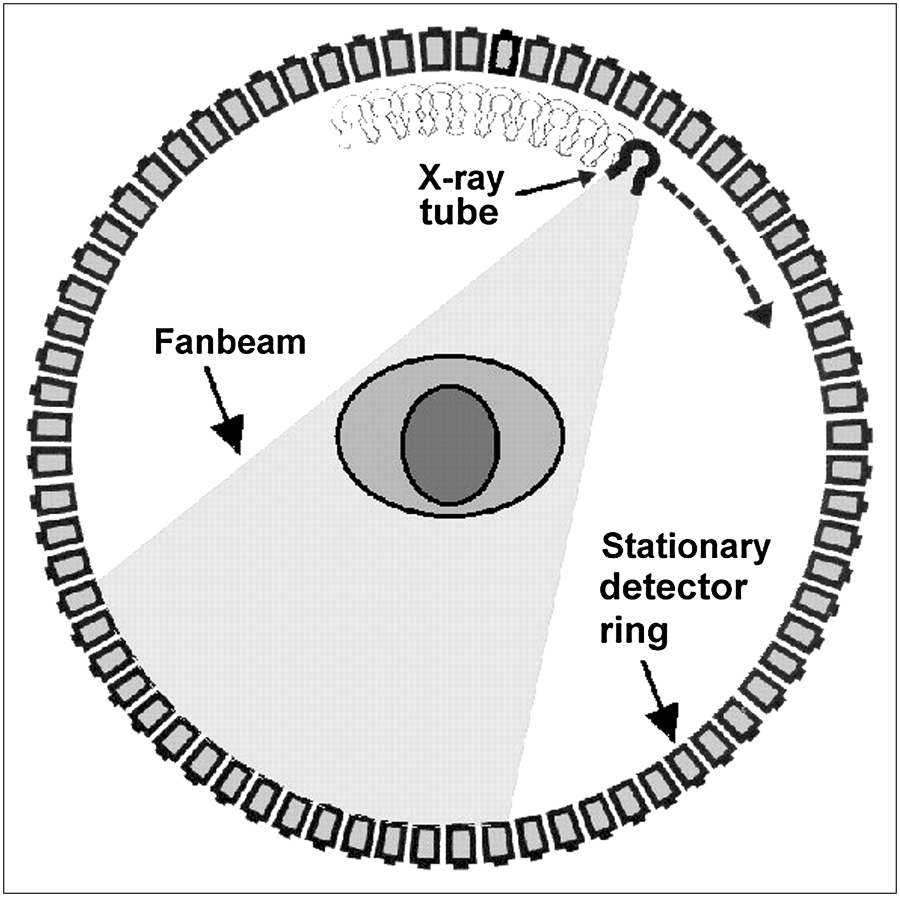
Faster scans required the elimination of translation motion and the use of smoother and simpler pure rotational motion. This goal is accomplished by widening the x-ray beam into a fanbeam encompassing the entire patient width and using an array of detectors to intercept the beam (Fig. 8). The detector array is rigidly linked to the x-ray tube, so that both the tube and the detectors rotate together around the patient (a motion referred to as rotation–rotation). Many detectors are used (250 for the initial models and 750 or more in later designs) to allow a sufficient number of measurements to be made across the scan circle. This design, characterized by linked tube–detector arrays undergoing only rotational motion, is known as third-generation geometry. The early third-generation CT scanners, installed in late 1975, could scan in less than 5 s; current designs can scan as quickly as one third of a second for cardiac applications.

View larger version (28K): [in this window] [in a new window]   FIGURE 8.  Third-generation geometry. Time-consuming and mechanically complex translation motion was eliminated by opening x-rays into fanbeam. Large array of detectors measured data across width of fan. Tube and detectors were rigidly linked and underwent single rotational motion.

A solution was provided by xenon detector arrays (supplemental Fig. 8) (10). A xenon array consisted of a long metal chamber subdivided into many small chambers by thin plates called septa. Every second septum was connected to a common positive bias voltage source. The alternate septa acted as collectors individually connected to an electronic readout. Each small chamber thus formed an ionization detector (7). Xenon arrays were inherently stable and well matched because factors affecting detector responses were either uniform for the entire array (bias voltage or type and density of gas) or constant over time (chamber volume). Xenon (atomic number 54) under high pressure (10–25 atm, to increase density), rather than poorly absorbing air, was used to maximize the absorption of x-rays entering the detectors. Xenon arrays were eventually replaced by solid-state detectors (discussed later).

It should be noted than ring artifacts in third-generation CT images are never completely eliminated. Rather, they are minimized by high-quality detector design and frequent (daily) calibration scans. Residual ring artifacts in images are then removed by image-processing algorithms, without which rings would likely be seen in every CT image. Detector failure or drift may still cause ring artifacts to occasionally appear. Despite this and other limitations described in the next section (and despite the introduction of a faster fourth generation of CT), third-generation CT was highly successful and remains the basic geometry of most CT scanners manufactured today.

CT PERFORMANCE CRITERIA

A few concepts regarding CT radiation dose and image quality are mentioned here to allow meaningful discussions of the advantages and trade-offs of various CT designs.

Dose Efficiency
Sensitivity (the ability to visualize low-contrast structures) is limited by noise (quantum mottle), which is caused by use of a finite, limited number of primary x-rays to form the image. Maximum sensitivity for any given radiation dose requires capturing and using as high a fraction of the primary x-rays exiting the patient as possible. This concept is referred to as dose efficiency, and it involves 2 factors: geometric efficiency (fraction of transmitted x-rays interacting with active detector areas) and absorption efficiency (fraction of x-rays interacting with active detector areas that are actually captured). Geometric efficiency is reduced if some x-rays are absorbed before detection (such as in the front housing of detectors) or if some x-rays do not enter active areas of the detectors (such as by passing between detectors or striking inactive dividers between individual detectors). Absorption efficiency is reduced if some x-rays entering the detectors pass all the way through without being absorbed.

The scintillation detectors used in first- and second-generation CT were sized to intercept the entire exiting narrow beam and absorbed essentially 100% of available x-rays (100% dose efficient).

In contrast, xenon detector absorption efficiency was about 60%–70%. Geometric efficiency was reduced by x-ray absorption in the housing and by x-rays striking the septa edge on, so that overall dose efficiency was typically about 50%–60%. By the mid-1980s, improvements in technology allowed more dose-efficient solid detector arrays to begin replacing the xenon arrays used in third-generation scanners; solid detector arrays are the detectors of choice for all CT scanner manufacturers today.

Scatter
A fundamental advantage of the CT process was the potential to (almost) completely eliminate scatter. Scattered photons are emitted in (nearly) random directions (i.e., nearly isotropic). First-generation CT was essentially scatter-free, because only a very few scattered photons that happened to be scattered in directions nearly parallel to the narrow beam could reach the detectors.

In comparison, it seems that the broad fanbeam used in third-generation CT would reintroduce scatter carefully avoided in earlier generations. It is certainly true that more scatter is produced at any instant (because more tissue is irradiated) and that scatter that would miss a first-generation CT detector may be detected by a third-generation array (Fig. 9). However, the amount of scatter produced is still far less than that associated with conventional radiography, because the CT beam is not more than 1 cm wide in the Z direction, compared with up to 43 cm (17 in.) in radiography. In any case, even this scatter can be (mostly) eliminated by use of the equivalent of a scatter removal grid; x-ray-absorbing septa placed at the boundaries between detectors and aimed at the focal spot allow primary x-rays to pass while stopping most scattered x-rays before they enter the detectors (Fig. 9B).

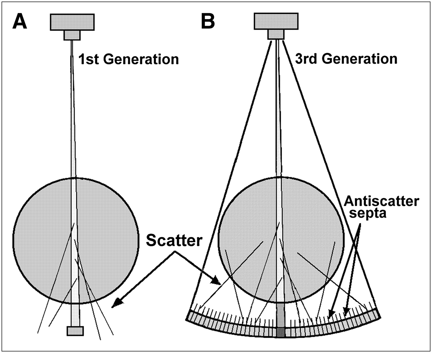
View larger version (38K): [in this window] [in a new window]   FIGURE 9.  Scatter with CT fanbeam. Use of fanbeam increases scatter production at any moment (more tissue is irradiated), and more scatter can reach detectors. Amount of scatter produced is still much smaller than that in radiography because fanbeam is only 1 cm thick. Scatter can be eliminated in third-generation CT with scatter removal septa, which act like nearly ideal grid. (A) First-generation CT. (B) Third-generation CT.

A limitation of third-generation geometry is this sampling. Although it is possible to collect views at any number of angles, sample size and spacing are fixed by detector design; samples cannot be closer together than the distance between rays associated with each detector at the level of the center of rotation (supplemental Fig. 9). Obtaining smaller and more closely spaced measurements would require a detector array with smaller—and more—detectors. A common technique for circumventing this limitation is the "1/4-ray offset." Suppose a scan is performed over 360° rather than 180°. At some point during the 360° scan, every ray is measured twice, but with the rays traveling in opposite directions. For example, a detector at the center of the array measures the same ray (i.e., x-rays passing through the same voxels) when the tube is at 0° and the detector is at 180° and again 180° later when their positions are reversed. Through a shift of the detector array mounting by a small amount (1/4 of a detector width) relative to the center of rotation, these opposing rays can be made to interleave, effectively doubling the sample density (i.e., the samples are half as far apart) (supplemental Fig. 10). An extension of this idea is the dynamic focal spot; although the tube and detectors are linked, the x-ray beam can move relative to the detectors through electronic shifting of the location of the focal spot on the x-ray tube anode. If the focal spot is shifted by half of a detector width, then interleaved samples are again obtained (11).

FOURTH-GENERATION SCANNERS

By 1976, 1-s scans were achieved with a design incorporating a large stationary ring of detectors, with the x-ray tube alone rotating around the patient (supplemental Fig. 11). This approach, known as fourth-generation geometry and developed under contract with the National Institutes of Health, is diagramed in Figure 10. Although it appeared later, fourth-generation technology was in fact developed (for the most part) in parallel with—and partly in response to—engineering challenges of the third-generation approach.

View larger version (55K): [in this window] [in a new window]   FIGURE 10.  Fourth-generation scan geometry. Fixed detector ring in original design was quite large, because tube rotated inside ring. Later designs moved tube outside ring and tilted ring out of way of x-ray beam as x-ray tube swept by.

Drawbacks of early fourth-generation CT included size and geometric dose efficiency. Because the tube rotated inside the detector ring, a large ring diameter (170–180 cm) was needed to maintain acceptable tube–skin distances. On the other hand, acceptable spatial resolution limited detector apertures to 4 mm. Consequently, even allowing for 10% space between detectors, 1,200 or more detectors were needed to fill the ring, but cost considerations initially limited the number to 600. The result was gaps between detectors and low geometric dose efficiency (<50%), as shown in supplemental Figure 11 (up to 4,800 detectors were eventually used). A later, alternate design used a smaller ring placed closer to the patient, with the tube rotating outside the ring; during tube rotation, the part of the ring between the tube and the patient would tilt out of the way of the x-ray beam (the peculiar wobbling motion of the ring was called nutation).

Another disadvantage of fourth-generation designs was scatter. The scatter-absorbing septa used in third-generation designs could not be used, because the septa would necessarily be aimed at the center of the ring, which was the source of the scatter (patient's location); that is, they would preferentially transmit scatter rather than primary x-rays. The removal of scatter was never truly solved in fourth-generation designs.

Although it was introduced later, fourth-generation CT was not more (or less) advanced than third-generation CT. Both had advantages and disadvantages, and both types of scanners were manufactured until relatively recently (although third-generation CT had a larger market share). It was only the advent of multislice CT, for which fourth-generation detector arrays would be prohibitively expensive, that led to the demise of fourth-generation CT.

ELECTRON-BEAM CT (EBCT)

Besides obvious mechanical challenges, subsecond scans would burden x-ray tubes; because approximately 250 mAs (i.e., tube current in milliamps times scan time in seconds) per slice are required for acceptable body CT, a "mere" 0.25-s scan would require sustaining 1,000 mA. However, cardiac CT requires ultrafast scans (<50 ms) to freeze cardiac motion, a goal unreachable with conventional scanning even today (although cardiac CT is possible with today's fastest multislice CT scanners assisted by gating and advanced image-processing software). Various ideas were proposed (including the use of multiple x-ray tubes), but the goal was ultimately accomplished with a novel CT design that had no moving parts and that was capable of performing complete scans in as little as 10–20 ms.

The idea behind ultrafast CT is a large, bell-shaped x-ray tube (supplemental Fig. 13) (12). An electron stream emitted from the cathode is focused into a narrow beam and electronically deflected to impinge on a small focal spot on an annular tungsten target anode, from which x-rays are then produced. The electron beam (and consequently the focal spot) is then electronically swept along all (or part) of the 360° circumference of the target. Wherever along the annular target the electron beam impinges, x-rays are generated and collimated into a fanbeam (various detector schemes were envisioned). The concept is known as EBCT.

A cardiac EBCT scanner with a partial (semicircular, 210°) anode and opposing detectors was built by 1984 (13). To acquire rapid heart scans without table (patient) movement, it included 4 anodes and 2 detector banks, each offset along the z-axis so as to acquire 8 interleaved slices covering 8 cm of the heart. Although the device was able to go faster, limited tube current (650 mA) required slower (50- to 100-ms) scans for acceptable mAs values and associated image quality (for a complete description of EBCT, see the chapter by McCollough in Medical CT and Ultrasound: Current Technologies and Applications (14)). Although still available, EBCT was limited to a niche market (cardiac screening), mostly because image quality for general scanning was lower than that of conventional CT (because of low mAs values) and because of higher equipment costs. With progress being made in cardiac scanning by multislice CT, the future of EBCT is uncertain.

SLIP RING SCANNERS AND HELICAL CT

After the fourth generation, CT technology remained stable (other than incremental improvements) until 1987. By then, CT examination times were dominated by interscan delays. After each 360° rotation, cables connecting rotating components (x-ray tube and, if third generation, detectors) to the rest of the gantry required that rotation stop and reverse direction. Cables were spooled onto a drum, released during rotation, and then respooled during reversal. Scanning, braking, and reversal required at least 8–10 s, of which only 1–2 were spent acquiring data. The result was poor temporal resolution (for dynamic contrast enhancement studies) and long procedure times.

Eliminating interscan delays required continuous (nonstop) rotation, a capability made possible by the low-voltage slip ring. A slip ring passes electrical power to the rotating components (e.g., x-ray tube and detectors) without fixed connections. The idea is similar to that used by bumper cars; power is passed to the cars through a metal brush that slides along a conductive ceiling. Similarly, a slip ring is a drum or annulus with grooves along which electrical contactor brushes slide (supplemental Fig. 14). Data are transmitted from detectors via various high-capacity wireless technologies, thus allowing continuous rotation to occur. A slip ring allows the complete elimination of interscan delays, except for the time required to move the table to the next slice position. However, the scan–move–scan sequence (known as axial step-and-shoot CT) is still somewhat inefficient. For example, if scanning and moving the table each take 1 s, only 50% of the time is spent acquiring data. Furthermore, rapid table movements may introduce "tissue jiggle" motion artifacts into the images.

An alternate strategy is to continuously rotate and continuously acquire data as the table (patient) is smoothly moved though the gantry; the resulting trajectory of the tube and detectors relative to the patient traces out a helical or spiral path (Fig. 11) (15,16). This powerful concept, referred to synonymously as helical CT or spiral CT, allows for rapid scans of entire z-axis regions of interest, in some cases within a single breath hold. So significant were improvements in body CT quality and throughput that helical scanning became the de facto standard of care for body CT by the mid-1990's.

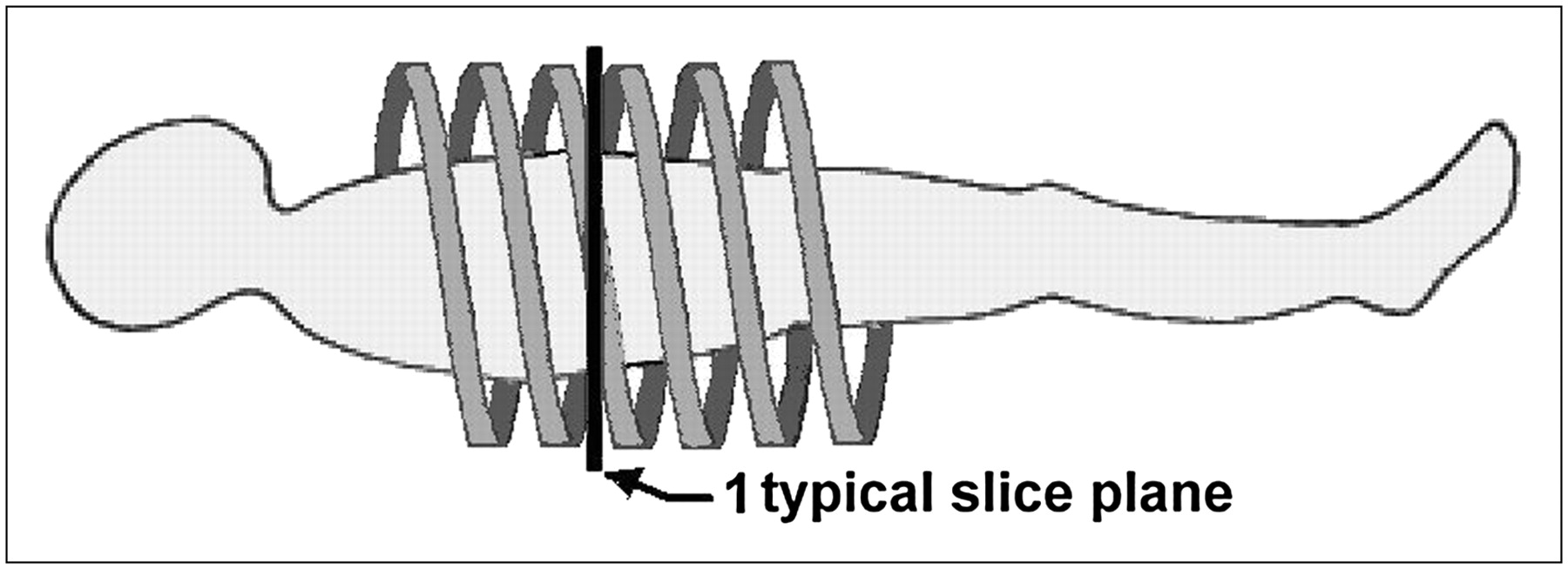
View larger version (20K): [in this window] [in a new window]   FIGURE 11.  Helical CT. Improved body CT was made possible with advent of helical CT (or spiral CT). Patient table is moved smoothly through gantry as rotation and data collection continue. Resulting data form spiral (or helical) path relative to patient; slices at arbitrary locations may be reconstructed from these data.

Another concept associated with helical CT is slice interpolation. For step-and-shoot CT, all data for slice reconstruction are collected at the Z position of that slice before moving to the next position. Reconstructed slices clearly correspond to the Z positions at which the data were obtained. Helical CT, however, provides no obvious slice Z positions; relative to the continuous helical data path, any arbitrarily selected slice plane (such as the vertical line in Fig. 11) is equivalent to any other. Thus, once helical data are acquired, slices may be reconstructed at any Z position. On the other hand, no slice plane contains sufficient data to actually reconstruct a slice. To see the problem, consider the slice plane shown as a vertical line in Fig. 11; if the helix represents the path of the detectors, then it is clear that the detectors (and thus the locations of measured views) are above the slice plane at 0° but below the slice plane 180° later (or vice versa). Only a small number of measurements actually lie exactly within the plane of the slice. Recall, however, that image reconstruction requires that a sufficient number of views over a sufficiently large angle (at least 180°) be obtained. To allow image reconstruction, it is necessary to estimate from the measurements lying above and below the slice what the measurements would have been within the slice. The process known as interpolation is used to make these estimates.

For example, suppose a scan is performed with a 10-mm slice thickness and a pitch of 1 and then data (rays) measured by one particular detector are considered. Suppose that when this detector is at 50° (i.e., it measures a ray whose path through the patient is at 50°), the detector is 5 mm above the plane of the slice to be reconstructed. After one rotation with a pitch of 1, that detector again measures a ray at 50° but now 5 mm below the desired plane. To estimate the equivalent 50° ray that would have been measured by this detector within the slice plane, interpolation between the measurements obtained 5 mm below and those obtained 5 mm above is used. In this case, because the 2 measurements are equidistant from the slice, the 2 measurements are simply averaged. If instead the first measurement is only 2 mm above the slice and the second measurement is 8 mm below, then the first measurement—being closer—is given greater weight.

It is distinctly possible, however, that the anatomy actually lying between the 2 measurements in the example just described differs significantly from that at which the measurements are obtained (there may be rapidly changing anatomy or small structures). If so, then the estimate may be significantly in error, leading to image misrepresentation or image artifacts. As a rule, the farther apart interpolated data points are, the greater the chance of error. The process just described is called 360° interpolation, because data are interpolated between measurements obtained 360° (one full rotation) apart by the same detector. However, this scheme can be improved; as noted earlier, at some point during each 360° rotation, every ray is measured twice, but with the x-rays traveling in opposite directions (i.e., 180° apart). These 180°-opposed rays are closer together—and thus allow fewer chances for interpolation errors—than those that are 360° apart. The process that makes use of these rays is known as 180° interpolation and is the one that is generally used (Fig. 12). (Note that it is only for detectors at the center of the array that 180°-opposed rays are exactly half as far apart as those separated by 360°; for detectors closer to the ends of the array, measurements will not be as evenly spaced.)

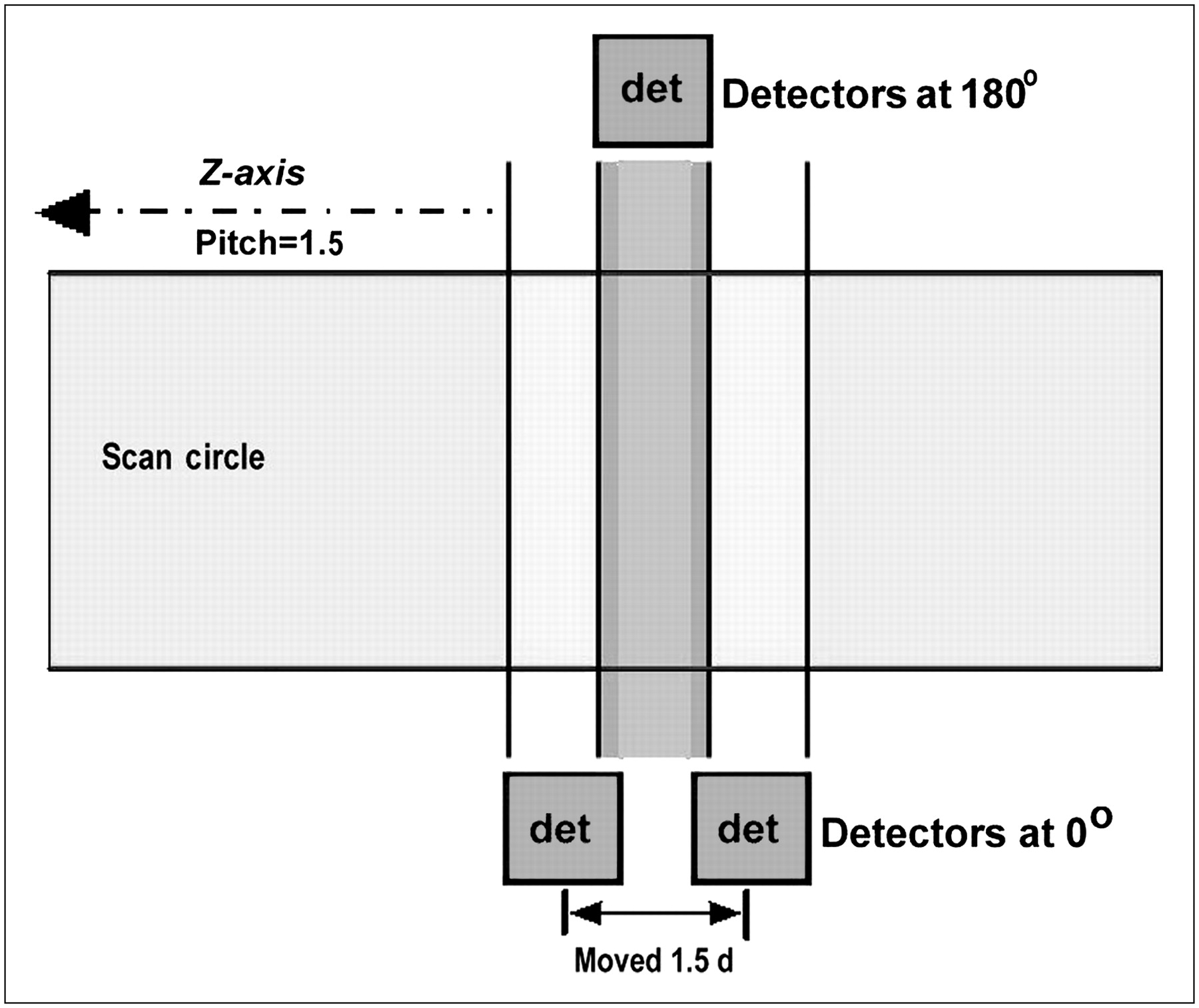
View larger version (23K): [in this window] [in a new window]   FIGURE 12.  Helical CT sample spacing and interpolation. If data for desired slice of thickness d (dark gray bar in figure) are interpolated between equivalent rays from adjacent helical rotations (loops) with pitch of 1.5, samples will be 1.5 d apart along z-axis (e.g., 10.5 mm apart for 7-mm thickness). Larger spacing means greater chance that interpolated estimate is in error. If 180°-opposed rays are included, measurements average half as far apart (and are more likely to actually lie within slice). det = detector.

The definition of pitch described earlier (table movement per rotation divided by the slice thickness) has been altered to accommodate multislice CT. The definition has been updated by replacing slice thickness in the denominator with the z-axis x-ray beam width. However, for conventional single-slice CT, slice thickness and z-axis x-ray beam width are equivalent.

CT FLUOROSCOPY

The potential for the high sensitivity of CT to guide percutaneous aspirations and biopsies had long been recognized. With continuous, dynamic scanning being made possible by slip ring CT, real-time CT fluoroscopy became feasible. A slip ring scanner is modified to allow real-time tableside image viewing and table positioning via foot pedal–controlled acquisitions and joy stick–controlled table positioning. Because a slip ring scanner can continuously acquire views at a fixed z-axis, temporal resolution can be considerably better than expected on the basis of rotation speed; images can be updated several times per second by continually adding new data to the reconstruction dataset and dropping the oldest data. For example, suppose a first image is displayed after one full 360° rotation with a 1-s rotation time. After another 1/6 s, another 60° of views has been acquired and is added to the dataset, and the original 60° of data is dropped. A new image is displayed on the basis of the latest 360° (in this case, from data collected between 60° and 420°) but is 1/6 s later than the first image. After another 1/6 s, the image is again updated, from data collected between 120° and 480°, and so forth. Images are thus updated at 6 frames per second.

CT fluoroscopy has proven valuable for interventional procedures but creates the potential for significant radiation doses if too many images are acquired at a given location (17). To minimize radiation exposure, a recent trend has been to replace continuous acquisition with a series of discrete, rapidly acquired images to guide biopsies.

APPENDIX

To understand how each measurement can be reduced to a sum of the attenuation values in the voxels along the path of a ray, consider the row of voxels in Figure 3, where N_o is x-ray intensity entering the row of voxels, N_i is the detector-measured intensity, w_i is the path length of the ray through the voxel, and µ_i is the attenuation coefficient of the material contained within that voxel.

Consider the intensity N₁ exiting the first voxel (attenuation µ₁). Using the expression for exponential attenuation,

(Eq. 1A)

Similarly, given that the intensity N₁ enters the second voxel, the intensity exiting the second voxel is given by the following equation:

(Eq. 2A)

Given that N₂ enters the third voxel, the intensity exiting the third voxel is calculated as follows:

(Eq. 3A)

Proceeding in this fashion through the last voxel,

(Eq. 4A)

Because the product of exponential functions is equal to the sum of the exponents,

(Eq. 5A)

Dividing both sides by N_o, taking the natural logarithm of each side, and dividing by –1 yields the following equation:

(Eq. 6A)

N_i is the measurement obtained by the detector for this ray, and N_o is known from in-air reference detector measurements or from prior calibration scans. The left side of Equation 6A is designated the processed data point N_i'. Each term w_iµ_i represents the attenuation occurring within voxel i, which is designated u_i, yielding the following equation:

(Eq. 7A)

For the ray shown in Figure 3, w_i is the voxel width W and is equal for all voxels. However, in the more general case for other angles, a ray may pass through a voxel at an angle or only partially through a voxel, so that w_i will differ for each voxel. In any case, because voxel size as well as the path of each ray is known, w_i can be calculated and the attenuation coefficient µ_i of voxel can be determined.

FOOTNOTES

^* NOTE: FOR CE CREDIT, YOU CAN ACCESS THIS ACTIVITY THROUGH THE SNM WEB SITE (http://www.snm.org/ce_online) THROUGH SEPTEMBER 2009.

COPYRIGHT © 2007 by the Society of Nuclear Medicine, Inc.

References

1. Seibert JA, Boone JM. X-ray imaging physics for nuclear medicine technologists, part 2: x-ray interactions and image formation. J Nucl Med Technol. 2005;33:3–18.[Abstract/Free Full Text]
2. Bocage AEM. Procede et dispositifs de radiographie sur plaque en mouvement. French patent 536464.
3. Webb S. Historical experiments predating commercially available computed tomography. Br J Radiol. 1992;65:835–837.[Abstract/Free Full Text]
4. Hounsfield GN. Historical notes on computerized axial tomography. J Can Assoc Radiol. 1976;27:135–142.[Medline]
5. Bull J. History of computed tomography. In: Newton TH, Potts DG, eds. Technical Aspects of Computed Tomography. St. Louis, MO: C.V. Mosby Co.; 1981:3835–3849.
6. Hounsfield GN. Computerized transverse axial scanning (tomography), part 1: description of system. Br J Radiol. 1973;46:1016–1022.[Abstract/Free Full Text]
7. Introduction to Computed Tomography. General Electric Co.; 1976.
8. Ledley RS, Di Chiro G, Luessenhop AJ, Twigg HL. Computerized transaxial x-ray tomography of the human body. Science. 1974;186:207–221.[Abstract/Free Full Text]
9. Ketteringham J, Gempel P. History of computed tomography: 1967–1978—excerpts from an ongoing study for the National Science Foundation. Cambridge, MA: Arthur D. Little, Inc.; 1978.
10. Boyd D, Coonrod J, Denhart J, et al. A high pressure xenon proportional chamber for x-ray laminographic reconstruction using fan beam geometry. IEEE Trans Nucl Sci. 1974;21:184–187.
11. Sohval AR, Freundlich D. Plural source computed tomography device with improved resolution. U.S. patent 4 637 040. 1986.
12. Iinuma TA, Tateno Y, Umegaki Y, Watanabe E. Proposed system for ultrafast computed tomography. J Comput Assist Tomogr. 1977;1:494–499.[Medline]
13. Boyd DP, Gould RG, Quinn JR, et al. A proposed dynamic cardiac 3-D densitometer for early detection and evaluation of heart disease. IEEE Trans Nucl Sci. 1979;NS-26:2724–2727.[CrossRef]
14. McCollough CH. Principles and performance of electron beam CT. In: Goldman LW, Fowlkes JB, eds. Medical CT and Ultrasound: Current Technologies and Applications. Madison, WI: Advanced Medical Publishing; 1995:487–518.
15. Kalender WA, Seissler W, Klotz E, Vock P. Spiral volumetric CT with single-breath-hold technique, continuous transport and scanner rotation. Radiology. 1990;176:181–183.[Abstract/Free Full Text]
16. Toki Y. Principles of helical scanning. In: Kimura K, Koga S, eds. Basic Principles and Clinical Applications of Helical Scan: Application of Continuous Rotation CT. Tokyo, Japan: Iryokagakusha; 1993:110–120.
17. Silverman SG, Tuncali K, Douglass FA, et al. CT fluoroscopy-guided abdominal interventions: techniques, results and radiation exposure. Radiology. 1999;212:673–681.[Abstract/Free Full Text]

This article has been cited by other articles:

				L. W. Goldman Principles of CT: Multislice CT J. Nucl. Med. Technol., June 1, 2008; 36(2): 57 - 68. [Abstract] [Full Text] [PDF]

				L. W. Goldman Principles of CT: Radiation Dose and Image Quality J. Nucl. Med. Technol., December 1, 2007; 35(4): 213 - 225. [Abstract] [Full Text] [PDF]

This Article Abstract Figures Only Full Text (PDF) CME Activity Supplemental Data Alert me when this article is cited Alert me if a correction is posted Services Email this article to a friend Similar articles in this journal Similar articles in PubMed Alert me to new issues of the journal Download to citation manager Citing Articles Citing Articles via HighWire Citing Articles via Google Scholar Google Scholar Articles by Goldman, L. W. Search for Related Content PubMed PubMed Citation Articles by Goldman, L. W.

References

- Received for publication April 23, 2007.
- Accepted for publication May 7, 2007.
Jump to section