


Abstract
This article is the second part of a continuing education series reviewing basic statistics that nuclear medicine and molecular imaging technologists should understand. In this article, the statistics for evaluating interpretation accuracy, significance, and variance are discussed. Throughout the article, actual statistics are pulled from the published literature. We begin by explaining 2 methods for quantifying interpretive accuracy: interreader and intrareader reliability. Agreement among readers can be expressed simply as a percentage. However, the Cohen κ-statistic is a more robust measure of agreement that accounts for chance. The higher the κ-statistic is, the higher is the agreement between readers. When 3 or more readers are being compared, the Fleiss κ-statistic is used. Significance testing determines whether the difference between 2 conditions or interventions is meaningful. Statistical significance is usually expressed using a number called a probability (P) value. Calculation of P value is beyond the scope of this review. However, knowing how to interpret P values is important for understanding the scientific literature. Generally, a P value of less than 0.05 is considered significant and indicates that the results of the experiment are due to more than just chance. Variance, standard deviation (SD), confidence interval, and standard error (SE) explain the dispersion of data around a mean of a sample drawn from a population. SD is commonly reported in the literature. A small SD indicates that there is not much variation in the sample data. Many biologic measurements fall into what is referred to as a normal distribution taking the shape of a bell curve. In a normal distribution, 68% of the data will fall within 1 SD, 95% will fall within 2 SDs, and 99.7% will fall within 3 SDs. Confidence interval defines the range of possible values within which the population parameter is likely to lie and gives an idea of the precision of the statistic being measured. A wide confidence interval indicates that if the experiment were repeated multiple times on other samples, the measured statistic would lie within a wide range of possibilities. The confidence interval relies on the SE.
- research methods
- statistical analysis
- statistics
- accuracy
- standard deviation
- statistics
- technologist
- variance
In this 2-part continuing education series, part 1 reviewed the statistics important in describing the accuracy of a diagnostic procedure—in other words, expressing how well a test distinguishes between 2 conditions, such as whether disease is present or disease is absent. The ability of a diagnostic test to discriminate is quantified by measures of diagnostic accuracy including sensitivity, specificity, accuracy, positive predictive value, negative predictive value, pretest probability, and posttest probability.
This second part of the series will review several additional statistical concepts with which molecular technologists should be familiar. First, accuracy of interpretation will be discussed. Interpretive accuracy is based on the level of consistency or agreement between observers: interreader reliability and intrareader reliability. In addition, hypothesis testing and significance will be briefly discussed. Significance testing determines whether differences between 2 tests are meaningful or are due to chance. Finally, some less fascinating but crucial statistics will be described, including variance, standard deviation (SD), confidence interval, and standard error (SE).
Examples from the nuclear medicine and molecular imaging literature are used to illustrate each statistical concept. It is hoped that the statistical concepts will be more easily understood when described in the context of real-world imaging.
ACCURACY OF INTERPRETATION
Interpretation issues must be considered when one is evaluating a molecular imaging test. How do you know whether an interpretation is accurate? How do you know whether the same interpreter would read a scan similarly if presented with it a second time? Does the test perform with the same sensitivity and specificity among different readers? How often do readers agree in their interpretation of the test?
Masked Interpretation
The best way for physicians to determine interpreter accuracy is to perform a masked-read experiment. Interpreters are considered “masked” when they are provided with the images alone, without any medical history, description of clinical symptoms, or other diagnostic testing information. The results of the masked interpretations are then compared with the known results.
For example, researchers looked at the sensitivity and specificity of 18F-florbetapir (Amyvid; Eli Lilly and Co), a PET amyloid imaging tracer, in the hands of multiple interpreters. Five independent and masked nuclear medicine physicians were asked to interpret 46 scans from patients who died within 12 mo of the amyloid PET study. The standard of truth for comparison was pathologic confirmation of amyloid plaque at autopsy, and the dataset included both positive and negative amyloid confirmations. The sensitivity of the majority reads across 5 readers was 96%, and specificity was 100%.
In the clinical patient-care setting, interpreters assume that, using the prescribed interpretation technique and acquiring images properly, the test performs as well for all interpreters as it did in the masked-read experiment.
Patient-specific or lesion-specific accuracy is difficult to measure in clinical practice without biopsy confirmation and often cannot be measured at all when the scan results are negative and no additional testing or follow-up is performed. Nuclear medicine physicians and radiologists can participate in hospital quality initiatives that systematically follow a group of patients and analyze outcomes against imaging results, thus measuring the readers’ own accuracy of interpretation. This is routinely done in mammography, for example. National mammography standards require that all radiologists who interpret mammography must do routine checks of accuracy (1). However, interpretation is more frequently assessed by comparing interpretations between 2 readers or within the same reader.
Interreader and Intrareader Reliability
Agreement among readers is also an important characteristic for a diagnostic test. How would you measure the level of agreement or disagreement among readers? If a scan has excellent accuracy with one expert reader but additional readers disagree about the findings, the test is less valuable. Interreader reliability is the measurement of how frequently interpreters agree with one another. The higher the reliability is, the higher is the agreement among readers and the more standardized the interpretation is across users. The lower the reliability is, the lower is the agreement among readers. Intrareader reliability is the measure of how consistently one reader interprets the same scan a second time. Ideally, intrareader reliability should be high, meaning that an interpreter reads the same scan the same way every time.
Agreement among a group of readers can be expressed as a percentage of the total reads. If 100 scans are interpreted by 2 readers who provide a binary result (e.g., positive or negative) and they disagree on 15 scans, the interreader agreement would be 85%. Reader agreement between 2 different tests can be evaluated in the same way. For example, 18F-fluciclovine researchers looked at the agreement between 18F-fluciclovine and 11C-choline PET interpretations in the same patients by analyzing results from 3 independent readers. Agreement between the 2 tests was 61% for reader 1, 67% for reader 2, and 77% for reader 3. Another way of stating the result is to say that the average agreement between the 2 tests among 3 readers was 68% (2). (Other ways of measuring interpreter performance are median read among interpreters or the average read result.)
Kappa (κ) Statistic
Reliability between 2 readers or within 1 reader can also be characterized by a correlation measure called the Cohen κ-statistic. This statistic measures agreement given the binary option of positive or negative. Considered to be a more robust measure of agreement than calculation of a simple percentage, the κ-statistic considers the fact that some agreement happens by chance (e.g., 2 readers may be guessing and happen to guess the same answer at the same time). The κ-statistic ranges from 0 (complete disagreement) to 1 (complete agreement), with a higher value indicating higher agreement and a lower value indicating lower agreement. Specifically, a κ-statistic of less than 0.20 indicates poor agreement (no more likely to occur than by chance; 0.21–0.40, fair agreement; 0.41–0.60, moderate agreement; 0.61–0.80, good agreement; 0.81–0.99, very good agreement; and 1.00, perfect agreement (3).
When 3 or more readers are evaluated, a similar statistic called the Fleiss κ-statistic is used. Like the Cohen κ-statistic, the closer the Fleiss κ-statistic is to 1.0, the closer is the interreader agreement to perfection (4).
A recent example of κ-measurement in the PET literature is a study by Ohira et al. (5) that looked at the interreader and intrareader reliability of 18F-FDG PET in patients being referred for evaluation of cardiac sarcoidosis. The authors measured agreement using 2 strategies: interpretation of uptake pattern (categories: focal uptake, focal on diffuse uptake, no uptake, diffuse uptake, or isolated lateral or basal uptake) and binary interpretation (positive or negative for cardiac sarcoidosis). The κ-statistic for pattern interpretation was 0.64, which reflect good agreement between 2 interpreters. The κ-statistic for binary interpretation was 0.85, showing a very good level of agreement between 2 interpreters. Analysis of intrareader agreement demonstrated very good agreement for both interpretation methods (0.94 for pattern interpretation and 0.92 for binary interpretation). These data help illustrate the impact of the 2 methods of interpretation on inter- and intrareader agreement.
SIGNIFICANCE
When 2 tests or interventions are compared, how can we know whether the data are meaningful? Statistical significance, usually represented by a number called the probability (P) value, is a way of making sure that the experimental result—the difference between 2 measurements—is not due to just chance. Calculation of P values is beyond the scope of this paper, but knowing how to interpret a P value is important for understanding the scientific literature. A P value that is less than 0.05 indicates that the results of the experiment are due to more than just chance. Put another way, the research hypothesis is that there is a difference between A and B, and the null hypothesis (generally the opposite of what you are interested in finding out) is that there is no difference between A and B. If the P value is less than 0.05, it means that the null hypothesis is rejected and the measured difference between A and B is most likely real. A P value larger than 0.05 means that not enough information is available to reject the null hypothesis and that, therefore, the measured difference between A and B could be due to random chance (6).
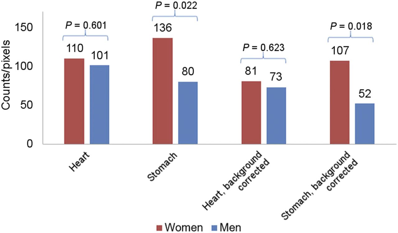
Figure 1 demonstrates P values and significance, using data from a previously published study (7). The investigators evaluated whether the aroma of hamburgers being cooked nearby would affect tracer uptake in the stomach on myocardial perfusion imaging. The bar graph shows that the count per pixel was higher in women than in men for both the stomach and the heart, but the P value reveals that this difference was statistically significant only for the stomach (background-corrected stomach, P = 0.018; background-corrected heart, P = 0.623). Therefore, the null hypothesis (i.e., no difference in stomach counts between women and men) must be rejected.

Demonstration of significant P values. Study evaluated tracer uptake in stomach during myocardial perfusion imaging when hamburgers were cooked nearby (7). Significant difference (significant P value) between women and men was found for stomach counts but not heart counts.
VARIANCE
To understand variance, SD, confidence intervals, and SE, imagine an experiment to calculate the average weight of male patients coming into your department for thyroid ablation. You collect data on 50 patients. The mean weight is 175 lb (1 lb = 0.45 kg), and the range is 100–250 lb. You could stop there and report the mean and range, but how reliable is that measurement and how confident are you that 175 lb is a good description of a typical patient in your sample? Figure 2 demonstrates how the distribution of weights can be very different although the mean is the same.
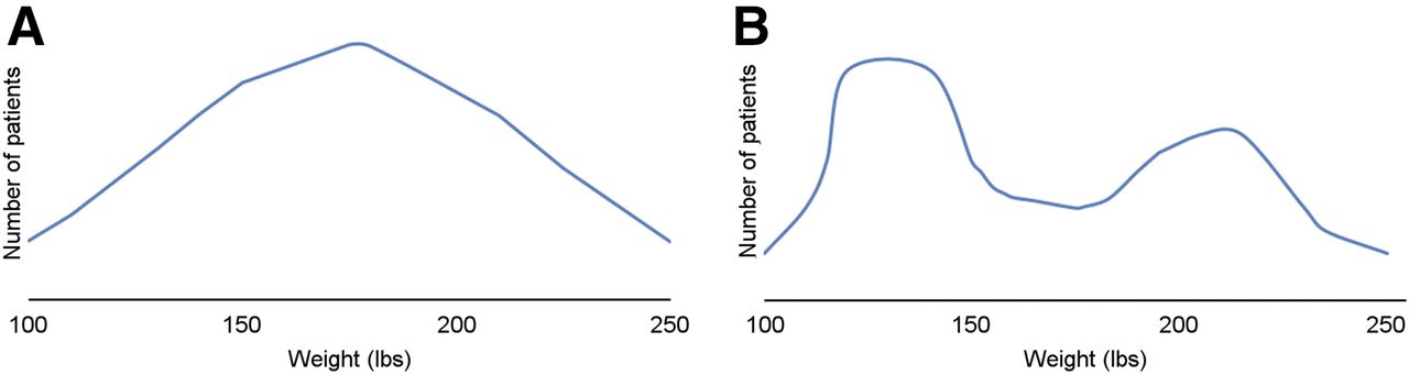
Graphs demonstrating variation in data for 2 samples although weight range (100–250 lb) and mean weight (175 lb) were the same for both populations: bell-shaped curve (A) and bimodal (2-peak) distribution (B).
To better characterize your data, the next step is to calculate the variance—how far from the mean your sample weights lie. The variance of a sample is the sum of all squared differences from the mean, divided by the sample size minus 1. To calculate the variance, the first step is to determine absolute differences from the mean for each patient. For the patient who weighed 100 lb, subtract 100 from 170 for a difference of 70 pounds, and 70 squared is 4,900. For the patient who weighed 250 lb, the difference from the mean is 170 − 250 lb, or 80 lb, and 80 squared is 6,400. After adding all the squared differences, divide the total by the sample size of 50 − 1 to determine the sample variation from the mean. For illustration’s sake, assume the sample variance is calculated as 35,839. As a stand-alone number, this is not useful to the average reader of statistics; however, this number is used in the determination of SD.
SD
SD, a commonly cited statistic in the medical literature, is used to measure the dispersion or variability in the sampling data. When we calculate the SD of a sample, we are using it as an estimate of the variability of the population from which the sample was drawn. A small SD indicates that there is not much variation in the sample data for this experiment and that the calculated statistic is a precise characterization of the sample. A large SD means that the data have a wide variability.
Mathematically, the SD of a sample equals the square root of the variance. In our weight experiment from above, the SD of our sample can be expressed as the square root of 35,839, or 26.8. This means that the sample mean and SD are 175 ± 26.8 lb.
Biologic measurements, such as weight, fall into what is referred to as a normal distribution. This means that if you plot the data from an infinite number of samples, the results will take the form of a standard curve, referred to as a bell curve because of its shape. The mean of the group will form the peak of the curve, and all other data will cluster around that mean in a predictable pattern. In a normal distribution, 95% of the data will fall within 1.96 SDs of the mean (usually rounded up to 2), and the remaining 5% will be scattered at the low or high end of the range (Fig. 3). Using our patient weight example above, we know that 95% of patients will fall within approximately 2 SDs, or 53.6 lb (26.7 × 2) above and 53.6 lb below. Therefore, an accurate description of a typical patient in the sample is between 116.4 and 223.6 lb. Note that, in this particular example, describing the population using a range (i.e., 100–250 lb), although accurate, is not as useful as describing the average plus the SD. Both statistics are accurate, but one is more meaningful to the researcher.
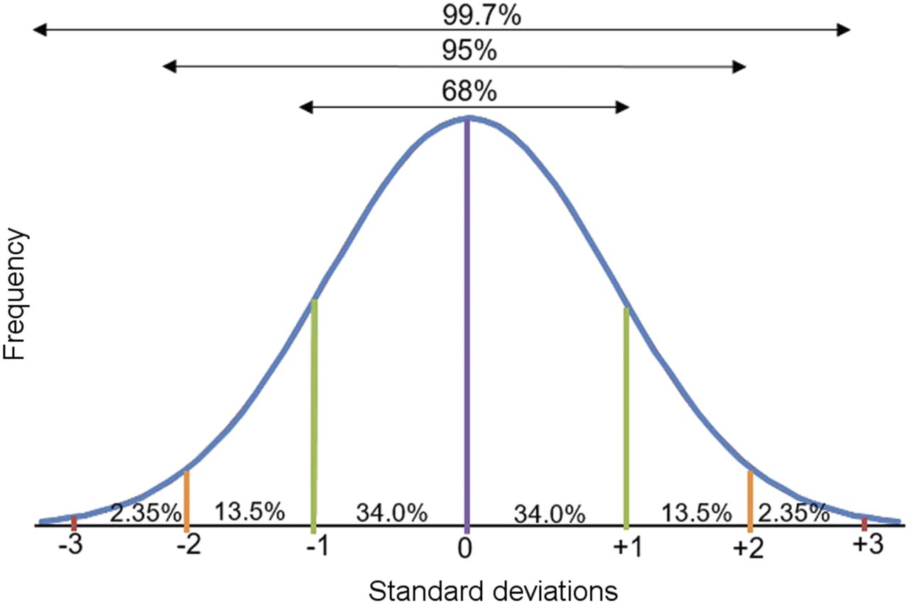
Normal bell-shaped distribution of data. Peak of curve is mean (purple line). One SD below and above mean (green lines) represents 68% of data, 2 SDs below and above mean (orange lines) represent 95% of data, and 3 SDs below and above mean (red lines) represent 99.7% of data.
Confidence Interval
Confidence interval is another tool to help us to understand the strength of a statistic. What is the difference between confidence interval and SD? A confidence interval defines a range of possible values within which our population parameter is likely to lie and gives an idea of the precision of the statistic being measured. Although SD describes the attributes of the individual data points that go into the sample statistic, confidence interval describes the range of results that would occur if the experiment were repeated with a different sample of the population. A wide confidence interval indicates that, if the experiment were repeated multiple times on other samples, the measured statistic would lie within a wide range of possibilities, indicating a lack of precision in the measurement. A narrow confidence interval means that the result is relatively more precise and that if the experiment were repeated, the range of likely results would be close to the original calculation. Confidence interval can be applied to any statistic, such as mean or κ.
SE
Confidence interval relies on calculation of another metric, SE. SE (denoted as SE or SEM), like SD, is a measurement of variance or dispersion from the mean. Although SD describes the variation between individuals and the calculated sample mean, SE is a measurement of uncertainty in the mean statistic itself. Referring to our patient weight experiment above, the population of 50 patients is only a small sample of all patients who undergo thyroid ablation. The mean and SD of the weight are assumed to approximate the population as a whole, but if another hospital repeats the experiment, or if the experiment is repeated with 50 additional patients, the mean may be a different number. SE helps us understand how reliable the mean measurement of the sample is compared with the mean of the entire population. In other words, SE describes how much variation there would be in the calculated mean if the entire experiment were performed repeatedly and an average calculated every time. The SE is equal to the SD divided by the square root of the sample size. Using our patient weight experiment, we could calculate the SE as 26.8 divided by the square root of 50 (7.07), which equals 3.8. SE by itself is not typically an informative statistic and is rarely cited; however, SE provides an important basis for group statistics, for example, as part of a calculation of confidence interval (6,8).
The mathematic definition for 95% confidence interval is “(mean – 1.96 × SE) to (mean + 1.96 × SE).” Using our weight experiment as raw data, with a mean of 175 lb and an SE of 3.8, the 95% confidence limit for the calculated mean would be derived as follows: In this example, therefore, these confidence limits tell us that if we repeated our weight experiment 100 times, we could expect 95 experiments to result in a calculated mean of between 162.5 and 177.5 lb. Confidence intervals can be calculated for other percentages, such as 99% confidence or 90% confidence; however, most examples in the medical literature use a 95% confidence interval.
An example of published confidence intervals can be seen in the prescribing information for 18F-florbetapir (9). Interreader reliability was measured, and the resulting Fleiss κ-statistic was 0.83, with a 95% confidence interval of 0.78–0.88. The κ-statistic itself indicates very good agreement, and the confidence interval tell us that there is a 95% likelihood that repeated experiments will result in a κ-statistic within the range of 0.78–0.88 (good to very good agreement). If the κ-statistic for a hypothetical test were 0.83 but the confidence interval very wide (e.g., 0.4–0.9), there would be concern that repeating the experiment could result in a κ-statistic ranging from fair agreement (0.4) to very good agreement (0.9). In this way, confidence intervals help us to know how reliable the statistic would be if repeated.
Significance (P value) and confidence interval, although testing 2 different things, are strongly related. If the calculated 95% confidence interval for a difference between 2 groups or tests does not include zero, meaning the range does not extend from a negative value to a positive value (e.g., −0.60 to −0.1 or 0.02 to 0.30, the hypothesis test will be significant (e.g., P < 0.05). If the confidence interval includes zero (e.g., −0.3 to 0.4), then there will not be statistical significance in the comparison (e.g., P > 0.05). This is why confidence intervals sometimes contain more clinically relevant information than P values. Presenting a 95% confidence interval indicates whether the result is statistically significant at the 5% level, but it also provides important information about how well the measurement would hold up under repeated testing (8).
CONCLUSION
The goal of this continuing education series on basic statistics was to provide a refresher for nuclear medicine and molecular imaging technologists. The statistics reviewed are those that are commonly found in the literature and that technologists should understand. Part 1 of the series reviewed statistics used to describe the characteristics of diagnostic imaging tests: sensitivity, specificity, and predictive value. Part 2 has discussed statistics used to evaluate interpretation accuracy, significance, and variance. Throughout the series, actual statistics were pulled from the published literature in the hope that the statistical concepts would more easily come to life. It is possible that a third part may be added to this series reviewing more complex concepts such as difference testing, risk, correlation, and survival analysis.
DISCLOSURE
No potential conflict of interest relevant to this article was reported.
Footnotes
Published online Feb. 2, 2018.
CE credit: For CE credit, you can access the test for this article, as well as additional JNMT CE tests, online at https://www.snmmilearningcenter.org. Complete the test online no later than June 2021. Your online test will be scored immediately. You may make 3 attempts to pass the test and must answer 80% of the questions correctly to receive 1.0 CEH (Continuing Education Hour) credit. SNMMI members will have their CEH credit added to their VOICE transcript automatically; nonmembers will be able to print out a CE certificate upon successfully completing the test. The online test is free to SNMMI members; nonmembers must pay $15.00 by credit card when logging onto the website to take the test.
REFERENCES
- Received for publication November 5, 2017.
- Accepted for publication December 14, 2017.


